Yolov8-源码解析-二十一-

Yolov8 源码解析（二十一）

---

comments: true
description: Optimize your YOLO model's performance with the right settings and hyperparameters. Learn about training, validation, and prediction configurations.
keywords: YOLO, hyperparameters, configuration, training, validation, prediction, model settings, Ultralytics, performance optimization, machine learning

YOLO settings and hyperparameters play a critical role in the model's performance, speed, and accuracy. These settings and hyperparameters can affect the model's behavior at various stages of the model development process, including training, validation, and prediction.

Watch: Mastering Ultralytics YOLOv8: Configuration

Ultralytics commands use the following syntax:

!!! Example

=== "CLI"

    ```py
    yolo TASK MODE ARGS
    ```

=== "Python"

    ```py
    from ultralytics import YOLO

    # Load a YOLOv8 model from a pre-trained weights file
    model = YOLO("yolov8n.pt")

    # Run MODE mode using the custom arguments ARGS (guess TASK)
    model.MODE(ARGS)
    ```

Where:

• TASK (optional) is one of (detect, segment, classify, pose)
• MODE (required) is one of (train, val, predict, export, track)
• ARGS (optional) are arg=value pairs like imgsz=640 that override defaults.

Default ARG values are defined on this page from the cfg/defaults.yaml file.

Tasks

YOLO models can be used for a variety of tasks, including detection, segmentation, classification and pose. These tasks differ in the type of output they produce and the specific problem they are designed to solve.

• Detect: For identifying and localizing objects or regions of interest in an image or video.
• Segment: For dividing an image or video into regions or pixels that correspond to different objects or classes.
• Classify: For predicting the class label of an input image.
• Pose: For identifying objects and estimating their keypoints in an image or video.
• OBB: Oriented (i.e. rotated) bounding boxes suitable for satellite or medical imagery.

Argument	Default	Description
task	'detect'	Specifies the YOLO task to be executed. Options include detect for object detection, segment for segmentation, classify for classification, pose for pose estimation and OBB for oriented bounding boxes. Each task is tailored to specific types of output and problems within image and video analysis.

Tasks Guide

Modes

YOLO models can be used in different modes depending on the specific problem you are trying to solve. These modes include:

• Train: For training a YOLOv8 model on a custom dataset.
• Val: For validating a YOLOv8 model after it has been trained.
• Predict: For making predictions using a trained YOLOv8 model on new images or videos.
• Export: For exporting a YOLOv8 model to a format that can be used for deployment.
• Track: For tracking objects in real-time using a YOLOv8 model.
• Benchmark: For benchmarking YOLOv8 exports (ONNX, TensorRT, etc.) speed and accuracy.

Argument	Default	Description
mode	'train'	Specifies the mode in which the YOLO model operates. Options are train for model training, val for validation, predict for inference on new data, export for model conversion to deployment formats, track for object tracking, and benchmark for performance evaluation. Each mode is designed for different stages of the model lifecycle, from development through deployment.

Modes Guide

Train Settings

The training settings for YOLO models encompass various hyperparameters and configurations used during the training process. These settings influence the model's performance, speed, and accuracy. Key training settings include batch size, learning rate, momentum, and weight decay. Additionally, the choice of optimizer, loss function, and training dataset composition can impact the training process. Careful tuning and experimentation with these settings are crucial for optimizing performance.

Argument	Default	Description
model	None	Specifies the model file for training. Accepts a path to either a .pt pretrained model or a .yaml configuration file. Essential for defining the model structure or initializing weights.
data	None	Path to the dataset configuration file (e.g., coco8.yaml). This file contains dataset-specific parameters, including paths to training and validation data, class names, and number of classes.
epochs	100	Total number of training epochs. Each epoch represents a full pass over the entire dataset. Adjusting this value can affect training duration and model performance.
time	None	Maximum training time in hours. If set, this overrides the epochs argument, allowing training to automatically stop after the specified duration. Useful for time-constrained training scenarios.
patience	100	Number of epochs to wait without improvement in validation metrics before early stopping the training. Helps prevent overfitting by stopping training when performance plateaus.
batch	16	Batch size, with three modes: set as an integer (e.g., batch=16), auto mode for 60% GPU memory utilization (batch=-1), or auto mode with specified utilization fraction (batch=0.70).
imgsz	640	Target image size for training. All images are resized to this dimension before being fed into the model. Affects model accuracy and computational complexity.
save	True	Enables saving of training checkpoints and final model weights. Useful for resuming training or model deployment.
save_period	-1	Frequency of saving model checkpoints, specified in epochs. A value of -1 disables this feature. Useful for saving interim models during long training sessions.
cache	False	Enables caching of dataset images in memory (True/ram), on disk (disk), or disables it (False). Improves training speed by reducing disk I/O at the cost of increased memory usage.
device	None	Specifies the computational device(s) for training: a single GPU (device=0), multiple GPUs (device=0,1), CPU (device=cpu), or MPS for Apple silicon (device=mps).
workers	8	Number of worker threads for data loading (per RANK if Multi-GPU training). Influences the speed of data preprocessing and feeding into the model, especially useful in multi-GPU setups.
project	None	Name of the project directory where training outputs are saved. Allows for organized storage of different experiments.
name	None	Name of the training run. Used for creating a subdirectory within the project folder, where training logs and outputs are stored.
exist_ok	False	If True, allows overwriting of an existing project/name directory. Useful for iterative experimentation without needing to manually clear previous outputs.
pretrained	True	Determines whether to start training from a pretrained model. Can be a boolean value or a string path to a specific model from which to load weights. Enhances training efficiency and model performance.
optimizer	'auto'	Choice of optimizer for training. Options include SGD, Adam, AdamW, NAdam, RAdam, RMSProp etc., or auto for automatic selection based on model configuration. Affects convergence speed and stability.
verbose	False	Enables verbose output during training, providing detailed logs and progress updates. Useful for debugging and closely monitoring the training process.
seed	0	Sets the random seed for training, ensuring reproducibility of results across runs with the same configurations.
deterministic	True	Forces deterministic algorithm use, ensuring reproducibility but may affect performance and speed due to the restriction on non-deterministic algorithms.
single_cls	False	Treats all classes in multi-class datasets as a single class during training. Useful for binary classification tasks or when focusing on object presence rather than classification.
rect	False	Enables rectangular training, optimizing batch composition for minimal padding. Can improve efficiency and speed but may affect model accuracy.
cos_lr	False	Utilizes a cosine learning rate scheduler, adjusting the learning rate following a cosine curve over epochs. Helps in managing learning rate for better convergence.
close_mosaic	10	Disables mosaic data augmentation in the last N epochs to stabilize training before completion. Setting to 0 disables this feature.
resume	False	Resumes training from the last saved checkpoint. Automatically loads model weights, optimizer state, and epoch count, continuing training seamlessly.
amp	True	Enables Automatic Mixed Precision (AMP) training, reducing memory usage and possibly speeding up training with minimal impact on accuracy.
fraction	1.0	Specifies the fraction of the dataset to use for training. Allows for training on a subset of the full dataset, useful for experiments or when resources are limited.
profile	False	Enables profiling of ONNX and TensorRT speeds during training, useful for optimizing model deployment.
freeze	None	Freezes the first N layers of the model or specified layers by index, reducing the number of trainable parameters. Useful for fine-tuning or transfer learning.
lr0	0.01	Initial learning rate (i.e. SGD=1E-2, Adam=1E-3) . Adjusting this value is crucial for the optimization process, influencing how rapidly model weights are updated.
lrf	0.01	Final learning rate as a fraction of the initial rate = (lr0 * lrf), used in conjunction with schedulers to adjust the learning rate over time.
momentum	0.937	Momentum factor for SGD or beta1 for Adam optimizers, influencing the incorporation of past gradients in the current update.
weight_decay	0.0005	L2 regularization term, penalizing large weights to prevent overfitting.
warmup_epochs	3.0	Number of epochs for learning rate warmup, gradually increasing the learning rate from a low value to the initial learning rate to stabilize training early on.
warmup_momentum	0.8	Initial momentum for warmup phase, gradually adjusting to the set momentum over the warmup period.
warmup_bias_lr	0.1	Learning rate for bias parameters during the warmup phase, helping stabilize model training in the initial epochs.
box	7.5	Weight of the box loss component in the loss function, influencing how much emphasis is placed on accurately predicting bounding box coordinates.
cls	0.5	Weight of the classification loss in the total loss function, affecting the importance of correct class prediction relative to other components.
dfl	1.5	Weight of the distribution focal loss, used in certain YOLO versions for fine-grained classification.
pose	12.0	Weight of the pose loss in models trained for pose estimation, influencing the emphasis on accurately predicting pose keypoints.
kobj	2.0	Weight of the keypoint objectness loss in pose estimation models, balancing detection confidence with pose accuracy.
label_smoothing	0.0	Applies label smoothing, softening hard labels to a mix of the target label and a uniform distribution over labels, can improve generalization.
nbs	64	Nominal batch size for normalization of loss.
overlap_mask	True	Determines whether segmentation masks should overlap during training, applicable in instance segmentation tasks.
mask_ratio	4	Downsample ratio for segmentation masks, affecting the resolution of masks used during training.
dropout	0.0	Dropout rate for regularization in classification tasks, preventing overfitting by randomly omitting units during training.
val	True	Enables validation during training, allowing for periodic evaluation of model performance on a separate dataset.
plots	False	Generates and saves plots of training and validation metrics, as well as prediction examples, providing visual insights into model performance and learning progression.

!!! info "Note on Batch-size Settings"

The `batch` argument can be configured in three ways:

- **Fixed Batch Size**: Set an integer value (e.g., `batch=16`), specifying the number of images per batch directly.
- **Auto Mode (60% GPU Memory)**: Use `batch=-1` to automatically adjust batch size for approximately 60% CUDA memory utilization.
- **Auto Mode with Utilization Fraction**: Set a fraction value (e.g., `batch=0.70`) to adjust batch size based on the specified fraction of GPU memory usage.

Train Guide

Predict Settings

The prediction settings for YOLO models encompass a range of hyperparameters and configurations that influence the model's performance, speed, and accuracy during inference on new data. Careful tuning and experimentation with these settings are essential to achieve optimal performance for a specific task. Key settings include the confidence threshold, Non-Maximum Suppression (NMS) threshold, and the number of classes considered. Additional factors affecting the prediction process are input data size and format, the presence of supplementary features such as masks or multiple labels per box, and the particular task the model is employed for.

Inference arguments:

Argument	Type	Default	Description
source	str	'ultralytics/assets'	Specifies the data source for inference. Can be an image path, video file, directory, URL, or device ID for live feeds. Supports a wide range of formats and sources, enabling flexible application across different types of input.
conf	float	0.25	Sets the minimum confidence threshold for detections. Objects detected with confidence below this threshold will be disregarded. Adjusting this value can help reduce false positives.
iou	float	0.7	Intersection Over Union (IoU) threshold for Non-Maximum Suppression (NMS). Lower values result in fewer detections by eliminating overlapping boxes, useful for reducing duplicates.
imgsz	int or tuple	640	Defines the image size for inference. Can be a single integer 640 for square resizing or a (height, width) tuple. Proper sizing can improve detection accuracy and processing speed.
half	bool	False	Enables half-precision (FP16) inference, which can speed up model inference on supported GPUs with minimal impact on accuracy.
device	str	None	Specifies the device for inference (e.g., cpu, cuda:0 or 0). Allows users to select between CPU, a specific GPU, or other compute devices for model execution.
max_det	int	300	Maximum number of detections allowed per image. Limits the total number of objects the model can detect in a single inference, preventing excessive outputs in dense scenes.
vid_stride	int	1	Frame stride for video inputs. Allows skipping frames in videos to speed up processing at the cost of temporal resolution. A value of 1 processes every frame, higher values skip frames.
stream_buffer	bool	False	Determines if all frames should be buffered when processing video streams (True), or if the model should return the most recent frame (False). Useful for real-time applications.
visualize	bool	False	Activates visualization of model features during inference, providing insights into what the model is "seeing". Useful for debugging and model interpretation.
augment	bool	False	Enables test-time augmentation (TTA) for predictions, potentially improving detection robustness at the cost of inference speed.
agnostic_nms	bool	False	Enables class-agnostic Non-Maximum Suppression (NMS), which merges overlapping boxes of different classes. Useful in multi-class detection scenarios where class overlap is common.
classes	list[int]	None	Filters predictions to a set of class IDs. Only detections belonging to the specified classes will be returned. Useful for focusing on relevant objects in multi-class detection tasks.
retina_masks	bool	False	Uses high-resolution segmentation masks if available in the model. This can enhance mask quality for segmentation tasks, providing finer detail.
embed	list[int]	None	Specifies the layers from which to extract feature vectors or embeddings. Useful for downstream tasks like clustering or similarity search.

Visualization arguments:

Argument	Type	Default	Description
show	bool	False	If True, displays the annotated images or videos in a window. Useful for immediate visual feedback during development or testing.
save	bool	False	Enables saving of the annotated images or videos to file. Useful for documentation, further analysis, or sharing results.
save_frames	bool	False	When processing videos, saves individual frames as images. Useful for extracting specific frames or for detailed frame-by-frame analysis.
save_txt	bool	False	Saves detection results in a text file, following the format [class] [x_center] [y_center] [width] [height] [confidence]. Useful for integration with other analysis tools.
save_conf	bool	False	Includes confidence scores in the saved text files. Enhances the detail available for post-processing and analysis.
save_crop	bool	False	Saves cropped images of detections. Useful for dataset augmentation, analysis, or creating focused datasets for specific objects.
show_labels	bool	True	Displays labels for each detection in the visual output. Provides immediate understanding of detected objects.
show_conf	bool	True	Displays the confidence score for each detection alongside the label. Gives insight into the model's certainty for each detection.
show_boxes	bool	True	Draws bounding boxes around detected objects. Essential for visual identification and location of objects in images or video frames.
line_width	None or int	None	Specifies the line width of bounding boxes. If None, the line width is automatically adjusted based on the image size. Provides visual customization for clarity.

Predict Guide

Validation Settings

The val (validation) settings for YOLO models involve various hyperparameters and configurations used to evaluate the model's performance on a validation dataset. These settings influence the model's performance, speed, and accuracy. Common YOLO validation settings include batch size, validation frequency during training, and performance evaluation metrics. Other factors affecting the validation process include the validation dataset's size and composition, as well as the specific task the model is employed for.

Argument	Type	Default	Description
data	str	None	Specifies the path to the dataset configuration file (e.g., coco8.yaml). This file includes paths to validation data, class names, and number of classes.
imgsz	int	640	Defines the size of input images. All images are resized to this dimension before processing.
batch	int	16	Sets the number of images per batch. Use -1 for AutoBatch, which automatically adjusts based on GPU memory availability.
save_json	bool	False	If True, saves the results to a JSON file for further analysis or integration with other tools.
save_hybrid	bool	False	If True, saves a hybrid version of labels that combines original annotations with additional model predictions.
conf	float	0.001	Sets the minimum confidence threshold for detections. Detections with confidence below this threshold are discarded.
iou	float	0.6	Sets the Intersection Over Union (IoU) threshold for Non-Maximum Suppression (NMS). Helps in reducing duplicate detections.
max_det	int	300	Limits the maximum number of detections per image. Useful in dense scenes to prevent excessive detections.
half	bool	True	Enables half-precision (FP16) computation, reducing memory usage and potentially increasing speed with minimal impact on accuracy.
device	str	None	Specifies the device for validation (cpu, cuda:0, etc.). Allows flexibility in utilizing CPU or GPU resources.
dnn	bool	False	If True, uses the OpenCV DNN module for ONNX model inference, offering an alternative to PyTorch inference methods.
plots	bool	False	When set to True, generates and saves plots of predictions versus ground truth for visual evaluation of the model's performance.
rect	bool	False	If True, uses rectangular inference for batching, reducing padding and potentially increasing speed and efficiency.
split	str	val	Determines the dataset split to use for validation (val, test, or train). Allows flexibility in choosing the data segment for performance evaluation.

Careful tuning and experimentation with these settings are crucial to ensure optimal performance on the validation dataset and detect and prevent overfitting.

Val Guide

Export Settings

Export settings for YOLO models encompass configurations and options related to saving or exporting the model for use in different environments or platforms. These settings can impact the model's performance, size, and compatibility with various systems. Key export settings include the exported model file format (e.g., ONNX, TensorFlow SavedModel), the target device (e.g., CPU, GPU), and additional features such as masks or multiple labels per box. The export process may also be affected by the model's specific task and the requirements or constraints of the destination environment or platform.

Argument	Type	Default	Description
format	str	'torchscript'	Target format for the exported model, such as 'onnx', 'torchscript', 'tensorflow', or others, defining compatibility with various deployment environments.
imgsz	int or tuple	640	Desired image size for the model input. Can be an integer for square images or a tuple (height, width) for specific dimensions.
keras	bool	False	Enables export to Keras format for TensorFlow SavedModel, providing compatibility with TensorFlow serving and APIs.
optimize	bool	False	Applies optimization for mobile devices when exporting to TorchScript, potentially reducing model size and improving performance.
half	bool	False	Enables FP16 (half-precision) quantization, reducing model size and potentially speeding up inference on supported hardware.
int8	bool	False	Activates INT8 quantization, further compressing the model and speeding up inference with minimal accuracy loss, primarily for edge devices.
dynamic	bool	False	Allows dynamic input sizes for ONNX and TensorRT exports, enhancing flexibility in handling varying image dimensions.
simplify	bool	False	Simplifies the model graph for ONNX exports, potentially improving performance and compatibility.
opset	int	None	Specifies the ONNX opset version for compatibility with different ONNX parsers and runtimes. If not set, uses the latest supported version.
workspace	float	4.0	Sets the maximum workspace size in GB for TensorRT optimizations, balancing memory usage and performance.
nms	bool	False	Adds Non-Maximum Suppression (NMS) to the CoreML export, essential for accurate and efficient detection post-processing.

It is crucial to thoughtfully configure these settings to ensure the exported model is optimized for the intended use case and functions effectively in the target environment.

Export Guide

Augmentation Settings

Augmentation techniques are essential for improving the robustness and performance of YOLO models by introducing variability into the training data, helping the model generalize better to unseen data. The following table outlines the purpose and effect of each augmentation argument:

Argument	Type	Default	Range	Description
hsv_h	float	0.015	0.0 - 1.0	Adjusts the hue of the image by a fraction of the color wheel, introducing color variability. Helps the model generalize across different lighting conditions.
hsv_s	float	0.7	0.0 - 1.0	Alters the saturation of the image by a fraction, affecting the intensity of colors. Useful for simulating different environmental conditions.
hsv_v	float	0.4	0.0 - 1.0	Modifies the value (brightness) of the image by a fraction, helping the model to perform well under various lighting conditions.
degrees	float	0.0	-180 - +180	Rotates the image randomly within the specified degree range, improving the model's ability to recognize objects at various orientations.
translate	float	0.1	0.0 - 1.0	Translates the image horizontally and vertically by a fraction of the image size, aiding in learning to detect partially visible objects.
scale	float	0.5	>=0.0	Scales the image by a gain factor, simulating objects at different distances from the camera.
shear	float	0.0	-180 - +180	Shears the image by a specified degree, mimicking the effect of objects being viewed from different angles.
perspective	float	0.0	0.0 - 0.001	Applies a random perspective transformation to the image, enhancing the model's ability to understand objects in 3D space.
flipud	float	0.0	0.0 - 1.0	Flips the image upside down with the specified probability, increasing the data variability without affecting the object's characteristics.
fliplr	float	0.5	0.0 - 1.0	Flips the image left to right with the specified probability, useful for learning symmetrical objects and increasing dataset diversity.
bgr	float	0.0	0.0 - 1.0	Flips the image channels from RGB to BGR with the specified probability, useful for increasing robustness to incorrect channel ordering.
mosaic	float	1.0	0.0 - 1.0	Combines four training images into one, simulating different scene compositions and object interactions. Highly effective for complex scene understanding.
mixup	float	0.0	0.0 - 1.0	Blends two images and their labels, creating a composite image. Enhances the model's ability to generalize by introducing label noise and visual variability.
copy_paste	float	0.0	0.0 - 1.0	Copies objects from one image and pastes them onto another, useful for increasing object instances and learning object occlusion.
auto_augment	str	randaugment	-	Automatically applies a predefined augmentation policy (randaugment, autoaugment, augmix), optimizing for classification tasks by diversifying the visual features.
erasing	float	0.4	0.0 - 0.9	Randomly erases a portion of the image during classification training, encouraging the model to focus on less obvious features for recognition.
crop_fraction	float	1.0	0.1 - 1.0	Crops the classification image to a fraction of its size to emphasize central features and adapt to object scales, reducing background distractions.

These settings can be adjusted to meet the specific requirements of the dataset and task at hand. Experimenting with different values can help find the optimal augmentation strategy that leads to the best model performance.

Logging, Checkpoints and Plotting Settings

Logging, checkpoints, plotting, and file management are important considerations when training a YOLO model.

• Logging: It is often helpful to log various metrics and statistics during training to track the model's progress and diagnose any issues that may arise. This can be done using a logging library such as TensorBoard or by writing log messages to a file.
• Checkpoints: It is a good practice to save checkpoints of the model at regular intervals during training. This allows you to resume training from a previous point if the training process is interrupted or if you want to experiment with different training configurations.
• Plotting: Visualizing the model's performance and training progress can be helpful for understanding how the model is behaving and identifying potential issues. This can be done using a plotting library such as matplotlib or by generating plots using a logging library such as TensorBoard.
• File management: Managing the various files generated during the training process, such as model checkpoints, log files, and plots, can be challenging. It is important to have a clear and organized file structure to keep track of these files and make it easy to access and analyze them as needed.

Effective logging, checkpointing, plotting, and file management can help you keep track of the model's progress and make it easier to debug and optimize the training process.

Argument	Default	Description
project	'runs'	Specifies the root directory for saving training runs. Each run will be saved in a separate subdirectory within this directory.
name	'exp'	Defines the name of the experiment. If not specified, YOLO automatically increments this name for each run, e.g., exp, exp2, etc., to avoid overwriting previous experiments.
exist_ok	False	Determines whether to overwrite an existing experiment directory if one with the same name already exists. Setting this to True allows overwriting, while False prevents it.
plots	False	Controls the generation and saving of training and validation plots. Set to True to create plots such as loss curves, precision-recall curves, and sample predictions. Useful for visually tracking model performance over time.
save	False	Enables the saving of training checkpoints and final model weights. Set to True to periodically save model states, allowing training to be resumed from these checkpoints or models to be deployed.

FAQ

How do I improve the performance of my YOLO model during training?

Improving YOLO model performance involves tuning hyperparameters like batch size, learning rate, momentum, and weight decay. Adjusting augmentation settings, selecting the right optimizer, and employing techniques like early stopping or mixed precision can also help. For detailed guidance on training settings, refer to the Train Guide.

What are the key hyperparameters to consider for YOLO model accuracy?

Key hyperparameters affecting YOLO model accuracy include:

• Batch Size (batch): Larger batch sizes can stabilize training but may require more memory.
• Learning Rate (lr0): Controls the step size for weight updates; smaller rates offer fine adjustments but slow convergence.
• Momentum (momentum): Helps accelerate gradient vectors in the right directions, dampening oscillations.
• Image Size (imgsz): Larger image sizes can improve accuracy but increase computational load.

Adjust these values based on your dataset and hardware capabilities. Explore more in the Train Settings section.

How do I set the learning rate for training a YOLO model?

The learning rate (lr0) is crucial for optimization. A common starting point is 0.01 for SGD or 0.001 for Adam. It's essential to monitor training metrics and adjust if necessary. Use cosine learning rate schedulers (cos_lr) or warmup techniques (warmup_epochs, warmup_momentum) to dynamically modify the rate during training. Find more details in the Train Guide.

What are the default inference settings for YOLO models?

Default inference settings include:

• Confidence Threshold (conf=0.25): Minimum confidence for detections.
• IoU Threshold (iou=0.7): For Non-Maximum Suppression (NMS).
• Image Size (imgsz=640): Resizes input images prior to inference.
• Device (device=None): Selects CPU or GPU for inference.
  For a comprehensive overview, visit the Predict Settings section and the Predict Guide.

Why should I use mixed precision training with YOLO models?

Mixed precision training, enabled with amp=True, helps reduce memory usage and can speed up training by utilizing the advantages of both FP16 and FP32. This is beneficial for modern GPUs, which support mixed precision natively, allowing more models to fit in memory and enable faster computations without significant loss in accuracy. Learn more about this in the Train Guide.

---

comments: true
description: Explore the YOLOv8 command line interface (CLI) for easy execution of detection tasks without needing a Python environment.
keywords: YOLOv8 CLI, command line interface, YOLOv8 commands, detection tasks, Ultralytics, model training, model prediction

Command Line Interface Usage

The YOLO command line interface (CLI) allows for simple single-line commands without the need for a Python environment. CLI requires no customization or Python code. You can simply run all tasks from the terminal with the yolo command.

Watch: Mastering Ultralytics YOLOv8: CLI

!!! Example

=== "Syntax"

    Ultralytics `yolo` commands use the following syntax:
    ```py
    yolo TASK MODE ARGS

    Where   TASK (optional) is one of [detect, segment, classify]
            MODE (required) is one of [train, val, predict, export, track]
            ARGS (optional) are any number of custom 'arg=value' pairs like 'imgsz=320' that override defaults.
    ```
    See all ARGS in the full [Configuration Guide](cfg.md) or with `yolo cfg`

=== "Train"

    Train a detection model for 10 epochs with an initial learning_rate of 0.01
    ```py
    yolo train data=coco8.yaml model=yolov8n.pt epochs=10 lr0=0.01
    ```

=== "Predict"

    Predict a YouTube video using a pretrained segmentation model at image size 320:
    ```py
    yolo predict model=yolov8n-seg.pt source='https://youtu.be/LNwODJXcvt4' imgsz=320
    ```

=== "Val"

    Val a pretrained detection model at batch-size 1 and image size 640:
    ```py
    yolo val model=yolov8n.pt data=coco8.yaml batch=1 imgsz=640
    ```

=== "Export"

    Export a YOLOv8n classification model to ONNX format at image size 224 by 128 (no TASK required)
    ```py
    yolo export model=yolov8n-cls.pt format=onnx imgsz=224,128
    ```

=== "Special"

    Run special commands to see version, view settings, run checks and more:
    ```py
    yolo help
    yolo checks
    yolo version
    yolo settings
    yolo copy-cfg
    yolo cfg
    ```

Where:

• TASK (optional) is one of [detect, segment, classify]. If it is not passed explicitly YOLOv8 will try to guess the TASK from the model type.
• MODE (required) is one of [train, val, predict, export, track]
• ARGS (optional) are any number of custom arg=value pairs like imgsz=320 that override defaults. For a full list of available ARGS see the Configuration page and defaults.yaml

!!! Warning "Warning"

Arguments must be passed as `arg=val` pairs, split by an equals `=` sign and delimited by spaces ` ` between pairs. Do not use `--` argument prefixes or commas `,` between arguments.

- `yolo predict model=yolov8n.pt imgsz=640 conf=0.25`   ✅
- `yolo predict model yolov8n.pt imgsz 640 conf 0.25`   ❌
- `yolo predict --model yolov8n.pt --imgsz 640 --conf 0.25`   ❌

Train

Train YOLOv8n on the COCO8 dataset for 100 epochs at image size 640. For a full list of available arguments see the Configuration page.

!!! Example "Example"

=== "Train"

    Start training YOLOv8n on COCO8 for 100 epochs at image-size 640.
    ```py
    yolo detect train data=coco8.yaml model=yolov8n.pt epochs=100 imgsz=640
    ```

=== "Resume"

    Resume an interrupted training.
    ```py
    yolo detect train resume model=last.pt
    ```

Val

Validate trained YOLOv8n model accuracy on the COCO8 dataset. No argument need to passed as the model retains its training data and arguments as model attributes.

!!! Example "Example"

=== "Official"

    Validate an official YOLOv8n model.
    ```py
    yolo detect val model=yolov8n.pt
    ```

=== "Custom"

    Validate a custom-trained model.
    ```py
    yolo detect val model=path/to/best.pt
    ```

Predict

Use a trained YOLOv8n model to run predictions on images.

!!! Example "Example"

=== "Official"

    Predict with an official YOLOv8n model.
    ```py
    yolo detect predict model=yolov8n.pt source='https://ultralytics.com/images/bus.jpg'
    ```

=== "Custom"

    Predict with a custom model.
    ```py
    yolo detect predict model=path/to/best.pt source='https://ultralytics.com/images/bus.jpg'
    ```

Export

Export a YOLOv8n model to a different format like ONNX, CoreML, etc.

!!! Example "Example"

=== "Official"

    Export an official YOLOv8n model to ONNX format.
    ```py
    yolo export model=yolov8n.pt format=onnx
    ```

=== "Custom"

    Export a custom-trained model to ONNX format.
    ```py
    yolo export model=path/to/best.pt format=onnx
    ```

Available YOLOv8 export formats are in the table below. You can export to any format using the format argument, i.e. format='onnx' or format='engine'.

Format	format Argument	Model	Metadata	Arguments
PyTorch	-	yolov8n.pt	✅	-
TorchScript	torchscript	yolov8n.torchscript	✅	imgsz, optimize, batch
ONNX	onnx	yolov8n.onnx	✅	imgsz, half, dynamic, simplify, opset, batch
OpenVINO	openvino	yolov8n_openvino_model/	✅	imgsz, half, int8, batch
TensorRT	engine	yolov8n.engine	✅	imgsz, half, dynamic, simplify, workspace, int8, batch
CoreML	coreml	yolov8n.mlpackage	✅	imgsz, half, int8, nms, batch
TF SavedModel	saved_model	yolov8n_saved_model/	✅	imgsz, keras, int8, batch
TF GraphDef	pb	yolov8n.pb	❌	imgsz, batch
TF Lite	tflite	yolov8n.tflite	✅	imgsz, half, int8, batch
TF Edge TPU	edgetpu	yolov8n_edgetpu.tflite	✅	imgsz
TF.js	tfjs	yolov8n_web_model/	✅	imgsz, half, int8, batch
PaddlePaddle	paddle	yolov8n_paddle_model/	✅	imgsz, batch
NCNN	ncnn	yolov8n_ncnn_model/	✅	imgsz, half, batch

See full export details in the Export page.

Overriding default arguments

Default arguments can be overridden by simply passing them as arguments in the CLI in arg=value pairs.

!!! Tip ""

=== "Train"

    Train a detection model for `10 epochs` with `learning_rate` of `0.01`
    ```py
    yolo detect train data=coco8.yaml model=yolov8n.pt epochs=10 lr0=0.01
    ```

=== "Predict"

    Predict a YouTube video using a pretrained segmentation model at image size 320:
    ```py
    yolo segment predict model=yolov8n-seg.pt source='https://youtu.be/LNwODJXcvt4' imgsz=320
    ```

=== "Val"

    Validate a pretrained detection model at batch-size 1 and image size 640:
    ```py
    yolo detect val model=yolov8n.pt data=coco8.yaml batch=1 imgsz=640
    ```

Overriding default config file

You can override the default.yaml config file entirely by passing a new file with the cfg arguments, i.e. cfg=custom.yaml.

To do this first create a copy of default.yaml in your current working dir with the yolo copy-cfg command.

This will create default_copy.yaml, which you can then pass as cfg=default_copy.yaml along with any additional args, like imgsz=320 in this example:

!!! Example

=== "CLI"

    ```py
    yolo copy-cfg
    yolo cfg=default_copy.yaml imgsz=320
    ```

FAQ

How do I use the Ultralytics YOLOv8 command line interface (CLI) for model training?

To train a YOLOv8 model using the CLI, you can execute a simple one-line command in the terminal. For example, to train a detection model for 10 epochs with a learning rate of 0.01, you would run:

yolo train data=coco8.yaml model=yolov8n.pt epochs=10 lr0=0.01

This command uses the train mode with specific arguments. Refer to the full list of available arguments in the Configuration Guide.

What tasks can I perform with the Ultralytics YOLOv8 CLI?

The Ultralytics YOLOv8 CLI supports a variety of tasks including detection, segmentation, classification, validation, prediction, export, and tracking. For instance:

• Train a Model: Run yolo train data=<data.yaml> model=<model.pt> epochs=<num>.
• Run Predictions: Use yolo predict model=<model.pt> source=<data_source> imgsz=<image_size>.
• Export a Model: Execute yolo export model=<model.pt> format=<export_format>.

Each task can be customized with various arguments. For detailed syntax and examples, see the respective sections like Train, Predict, and Export.

How can I validate the accuracy of a trained YOLOv8 model using the CLI?

To validate a YOLOv8 model's accuracy, use the val mode. For example, to validate a pretrained detection model with a batch size of 1 and image size of 640, run:

yolo val model=yolov8n.pt data=coco8.yaml batch=1 imgsz=640

This command evaluates the model on the specified dataset and provides performance metrics. For more details, refer to the Val section.

What formats can I export my YOLOv8 models to using the CLI?

YOLOv8 models can be exported to various formats such as ONNX, CoreML, TensorRT, and more. For instance, to export a model to ONNX format, run:

yolo export model=yolov8n.pt format=onnx

For complete details, visit the Export page.

How do I customize YOLOv8 CLI commands to override default arguments?

To override default arguments in YOLOv8 CLI commands, pass them as arg=value pairs. For example, to train a model with custom arguments, use:

yolo train data=coco8.yaml model=yolov8n.pt epochs=10 lr0=0.01

For a full list of available arguments and their descriptions, refer to the Configuration Guide. Ensure arguments are formatted correctly, as shown in the Overriding default arguments section.

---

comments: true
description: Learn to customize the YOLOv8 Trainer for specific tasks. Step-by-step instructions with Python examples for maximum model performance.
keywords: Ultralytics, YOLOv8, Trainer Customization, Python, Machine Learning, AI, Model Training, DetectionTrainer, Custom Models

Both the Ultralytics YOLO command-line and Python interfaces are simply a high-level abstraction on the base engine executors. Let's take a look at the Trainer engine.

Watch: Mastering Ultralytics YOLOv8: Advanced Customization

BaseTrainer

BaseTrainer contains the generic boilerplate training routine. It can be customized for any task based over overriding the required functions or operations as long the as correct formats are followed. For example, you can support your own custom model and dataloader by just overriding these functions:

• get_model(cfg, weights) - The function that builds the model to be trained
• get_dataloader() - The function that builds the dataloader More details and source code can be found in BaseTrainer Reference

DetectionTrainer

Here's how you can use the YOLOv8 DetectionTrainer and customize it.

from ultralytics.models.yolo.detect import DetectionTrainer

trainer = DetectionTrainer(overrides={...})
trainer.train()
trained_model = trainer.best  # get best model

Customizing the DetectionTrainer

Let's customize the trainer to train a custom detection model that is not supported directly. You can do this by simply overloading the existing the get_model functionality:

from ultralytics.models.yolo.detect import DetectionTrainer


class CustomTrainer(DetectionTrainer):
    def get_model(self, cfg, weights):
        """Loads a custom detection model given configuration and weight files."""
        ...


trainer = CustomTrainer(overrides={...})
trainer.train()

You now realize that you need to customize the trainer further to:

• Customize the loss function.
• Add callback that uploads model to your Google Drive after every 10 epochs Here's how you can do it:

from ultralytics.models.yolo.detect import DetectionTrainer
from ultralytics.nn.tasks import DetectionModel


class MyCustomModel(DetectionModel):
    def init_criterion(self):
        """Initializes the loss function and adds a callback for uploading the model to Google Drive every 10 epochs."""
        ...


class CustomTrainer(DetectionTrainer):
    def get_model(self, cfg, weights):
        """Returns a customized detection model instance configured with specified config and weights."""
        return MyCustomModel(...)


# callback to upload model weights
def log_model(trainer):
    """Logs the path of the last model weight used by the trainer."""
    last_weight_path = trainer.last
    print(last_weight_path)


trainer = CustomTrainer(overrides={...})
trainer.add_callback("on_train_epoch_end", log_model)  # Adds to existing callback
trainer.train()

To know more about Callback triggering events and entry point, checkout our Callbacks Guide

Other engine components

There are other components that can be customized similarly like Validators and Predictors. See Reference section for more information on these.

FAQ

How do I customize the Ultralytics YOLOv8 DetectionTrainer for specific tasks?

To customize the Ultralytics YOLOv8 DetectionTrainer for a specific task, you can override its methods to adapt to your custom model and dataloader. Start by inheriting from DetectionTrainer and then redefine methods like get_model to implement your custom functionalities. Here's an example:

from ultralytics.models.yolo.detect import DetectionTrainer


class CustomTrainer(DetectionTrainer):
    def get_model(self, cfg, weights):
        """Loads a custom detection model given configuration and weight files."""
        ...


trainer = CustomTrainer(overrides={...})
trainer.train()
trained_model = trainer.best  # get best model

For further customization like changing the loss function or adding a callback, you can reference our Callbacks Guide.

What are the key components of the BaseTrainer in Ultralytics YOLOv8?

The BaseTrainer in Ultralytics YOLOv8 serves as the foundation for training routines and can be customized for various tasks by overriding its generic methods. Key components include:

• get_model(cfg, weights) to build the model to be trained.
• get_dataloader() to build the dataloader.

For more details on the customization and source code, see the BaseTrainer Reference.

How can I add a callback to the Ultralytics YOLOv8 DetectionTrainer?

You can add callbacks to monitor and modify the training process in Ultralytics YOLOv8 DetectionTrainer. For instance, here's how you can add a callback to log model weights after every training epoch:

from ultralytics.models.yolo.detect import DetectionTrainer


# callback to upload model weights
def log_model(trainer):
    """Logs the path of the last model weight used by the trainer."""
    last_weight_path = trainer.last
    print(last_weight_path)


trainer = DetectionTrainer(overrides={...})
trainer.add_callback("on_train_epoch_end", log_model)  # Adds to existing callbacks
trainer.train()

For further details on callback events and entry points, refer to our Callbacks Guide.

Why should I use Ultralytics YOLOv8 for model training?

Ultralytics YOLOv8 offers a high-level abstraction on powerful engine executors, making it ideal for rapid development and customization. Key benefits include:

• Ease of Use: Both command-line and Python interfaces simplify complex tasks.
• Performance: Optimized for real-time object detection and various vision AI applications.
• Customization: Easily extendable for custom models, loss functions, and dataloaders.

Learn more about YOLOv8's capabilities by visiting Ultralytics YOLO.

Can I use the Ultralytics YOLOv8 DetectionTrainer for non-standard models?

Yes, Ultralytics YOLOv8 DetectionTrainer is highly flexible and can be customized for non-standard models. By inheriting from DetectionTrainer, you can overload different methods to support your specific model's needs. Here's a simple example:

from ultralytics.models.yolo.detect import DetectionTrainer


class CustomDetectionTrainer(DetectionTrainer):
    def get_model(self, cfg, weights):
        """Loads a custom detection model."""
        ...


trainer = CustomDetectionTrainer(overrides={...})
trainer.train()

For more comprehensive instructions and examples, review the DetectionTrainer documentation.

---

comments: true
description: Learn to integrate YOLOv8 in Python for object detection, segmentation, and classification. Load, train models, and make predictions easily with our comprehensive guide.
keywords: YOLOv8, Python, object detection, segmentation, classification, machine learning, AI, pretrained models, train models, make predictions

Python Usage

Welcome to the YOLOv8 Python Usage documentation! This guide is designed to help you seamlessly integrate YOLOv8 into your Python projects for object detection, segmentation, and classification. Here, you'll learn how to load and use pretrained models, train new models, and perform predictions on images. The easy-to-use Python interface is a valuable resource for anyone looking to incorporate YOLOv8 into their Python projects, allowing you to quickly implement advanced object detection capabilities. Let's get started!

Watch: Mastering Ultralytics YOLOv8: Python

For example, users can load a model, train it, evaluate its performance on a validation set, and even export it to ONNX format with just a few lines of code.

!!! Example "Python"

```py
from ultralytics import YOLO

# Create a new YOLO model from scratch
model = YOLO("yolov8n.yaml")

# Load a pretrained YOLO model (recommended for training)
model = YOLO("yolov8n.pt")

# Train the model using the 'coco8.yaml' dataset for 3 epochs
results = model.train(data="coco8.yaml", epochs=3)

# Evaluate the model's performance on the validation set
results = model.val()

# Perform object detection on an image using the model
results = model("https://ultralytics.com/images/bus.jpg")

# Export the model to ONNX format
success = model.export(format="onnx")
```

Train

Train mode is used for training a YOLOv8 model on a custom dataset. In this mode, the model is trained using the specified dataset and hyperparameters. The training process involves optimizing the model's parameters so that it can accurately predict the classes and locations of objects in an image.

!!! Example "Train"

=== "From pretrained(recommended)"

    ```py
    from ultralytics import YOLO

    model = YOLO("yolov8n.pt")  # pass any model type
    results = model.train(epochs=5)
    ```

=== "From scratch"

    ```py
    from ultralytics import YOLO

    model = YOLO("yolov8n.yaml")
    results = model.train(data="coco8.yaml", epochs=5)
    ```

=== "Resume"

    ```py
    model = YOLO("last.pt")
    results = model.train(resume=True)
    ```

Train Examples

Val

Val mode is used for validating a YOLOv8 model after it has been trained. In this mode, the model is evaluated on a validation set to measure its accuracy and generalization performance. This mode can be used to tune the hyperparameters of the model to improve its performance.

!!! Example "Val"

=== "Val after training"

    ```py
    from ultralytics import YOLO

    # Load a YOLOv8 model
    model = YOLO("yolov8n.yaml")

    # Train the model
    model.train(data="coco8.yaml", epochs=5)

    # Validate on training data
    model.val()
    ```

=== "Val on another dataset"

    ```py
    from ultralytics import YOLO

    # Load a YOLOv8 model
    model = YOLO("yolov8n.yaml")

    # Train the model
    model.train(data="coco8.yaml", epochs=5)

    # Validate on separate data
    model.val(data="path/to/separate/data.yaml")
    ```

Val Examples

Predict

Predict mode is used for making predictions using a trained YOLOv8 model on new images or videos. In this mode, the model is loaded from a checkpoint file, and the user can provide images or videos to perform inference. The model predicts the classes and locations of objects in the input images or videos.

!!! Example "Predict"

=== "From source"

    ```py
    import cv2
    from PIL import Image

    from ultralytics import YOLO

    model = YOLO("model.pt")
    # accepts all formats - image/dir/Path/URL/video/PIL/ndarray. 0 for webcam
    results = model.predict(source="0")
    results = model.predict(source="folder", show=True)  # Display preds. Accepts all YOLO predict arguments

    # from PIL
    im1 = Image.open("bus.jpg")
    results = model.predict(source=im1, save=True)  # save plotted images

    # from ndarray
    im2 = cv2.imread("bus.jpg")
    results = model.predict(source=im2, save=True, save_txt=True)  # save predictions as labels

    # from list of PIL/ndarray
    results = model.predict(source=[im1, im2])
    ```

=== "Results usage"

    ```py
    # results would be a list of Results object including all the predictions by default
    # but be careful as it could occupy a lot memory when there're many images,
    # especially the task is segmentation.
    # 1. return as a list
    results = model.predict(source="folder")

    # results would be a generator which is more friendly to memory by setting stream=True
    # 2. return as a generator
    results = model.predict(source=0, stream=True)

    for result in results:
        # Detection
        result.boxes.xyxy  # box with xyxy format, (N, 4)
        result.boxes.xywh  # box with xywh format, (N, 4)
        result.boxes.xyxyn  # box with xyxy format but normalized, (N, 4)
        result.boxes.xywhn  # box with xywh format but normalized, (N, 4)
        result.boxes.conf  # confidence score, (N, 1)
        result.boxes.cls  # cls, (N, 1)

        # Segmentation
        result.masks.data  # masks, (N, H, W)
        result.masks.xy  # x,y segments (pixels), List[segment] * N
        result.masks.xyn  # x,y segments (normalized), List[segment] * N

        # Classification
        result.probs  # cls prob, (num_class, )

    # Each result is composed of torch.Tensor by default,
    # in which you can easily use following functionality:
    result = result.cuda()
    result = result.cpu()
    result = result.to("cpu")
    result = result.numpy()
    ```

Predict Examples

Export

Export mode is used for exporting a YOLOv8 model to a format that can be used for deployment. In this mode, the model is converted to a format that can be used by other software applications or hardware devices. This mode is useful when deploying the model to production environments.

!!! Example "Export"

=== "Export to ONNX"

    Export an official YOLOv8n model to ONNX with dynamic batch-size and image-size.
    ```py
    from ultralytics import YOLO

    model = YOLO("yolov8n.pt")
    model.export(format="onnx", dynamic=True)
    ```

=== "Export to TensorRT"

    Export an official YOLOv8n model to TensorRT on `device=0` for acceleration on CUDA devices.
    ```py
    from ultralytics import YOLO

    model = YOLO("yolov8n.pt")
    model.export(format="onnx", device=0)
    ```

Export Examples

Track

Track mode is used for tracking objects in real-time using a YOLOv8 model. In this mode, the model is loaded from a checkpoint file, and the user can provide a live video stream to perform real-time object tracking. This mode is useful for applications such as surveillance systems or self-driving cars.

!!! Example "Track"

=== "Python"

    ```py
    from ultralytics import YOLO

    # Load a model
    model = YOLO("yolov8n.pt")  # load an official detection model
    model = YOLO("yolov8n-seg.pt")  # load an official segmentation model
    model = YOLO("path/to/best.pt")  # load a custom model

    # Track with the model
    results = model.track(source="https://youtu.be/LNwODJXcvt4", show=True)
    results = model.track(source="https://youtu.be/LNwODJXcvt4", show=True, tracker="bytetrack.yaml")
    ```

Track Examples

Benchmark

Benchmark mode is used to profile the speed and accuracy of various export formats for YOLOv8. The benchmarks provide information on the size of the exported format, its mAP50-95 metrics (for object detection and segmentation) or accuracy_top5 metrics (for classification), and the inference time in milliseconds per image across various export formats like ONNX, OpenVINO, TensorRT and others. This information can help users choose the optimal export format for their specific use case based on their requirements for speed and accuracy.

!!! Example "Benchmark"

=== "Python"

    Benchmark an official YOLOv8n model across all export formats.
    ```py
    from ultralytics.utils.benchmarks import benchmark

    # Benchmark
    benchmark(model="yolov8n.pt", data="coco8.yaml", imgsz=640, half=False, device=0)
    ```

Benchmark Examples

Explorer

Explorer API can be used to explore datasets with advanced semantic, vector-similarity and SQL search among other features. It also enabled searching for images based on their content using natural language by utilizing the power of LLMs. The Explorer API allows you to write your own dataset exploration notebooks or scripts to get insights into your datasets.

!!! Example "Semantic Search Using Explorer"

=== "Using Images"

    ```py
    from ultralytics import Explorer

    # create an Explorer object
    exp = Explorer(data="coco8.yaml", model="yolov8n.pt")
    exp.create_embeddings_table()

    similar = exp.get_similar(img="https://ultralytics.com/images/bus.jpg", limit=10)
    print(similar.head())

    # Search using multiple indices
    similar = exp.get_similar(
        img=["https://ultralytics.com/images/bus.jpg", "https://ultralytics.com/images/bus.jpg"], limit=10
    )
    print(similar.head())
    ```

=== "Using Dataset Indices"

    ```py
    from ultralytics import Explorer

    # create an Explorer object
    exp = Explorer(data="coco8.yaml", model="yolov8n.pt")
    exp.create_embeddings_table()

    similar = exp.get_similar(idx=1, limit=10)
    print(similar.head())

    # Search using multiple indices
    similar = exp.get_similar(idx=[1, 10], limit=10)
    print(similar.head())
    ```

Explorer

Using Trainers

YOLO model class is a high-level wrapper on the Trainer classes. Each YOLO task has its own trainer that inherits from BaseTrainer.

!!! Tip "Detection Trainer Example"

    ```py
    from ultralytics.models.yolo import DetectionPredictor, DetectionTrainer, DetectionValidator

    # trainer
    trainer = DetectionTrainer(overrides={})
    trainer.train()
    trained_model = trainer.best

    # Validator
    val = DetectionValidator(args=...)
    val(model=trained_model)

    # predictor
    pred = DetectionPredictor(overrides={})
    pred(source=SOURCE, model=trained_model)

    # resume from last weight
    overrides["resume"] = trainer.last
    trainer = detect.DetectionTrainer(overrides=overrides)
    ```

You can easily customize Trainers to support custom tasks or explore R&D ideas. Learn more about Customizing Trainers, Validators and Predictors to suit your project needs in the Customization Section.

Customization tutorials

FAQ

How can I integrate YOLOv8 into my Python project for object detection?

Integrating Ultralytics YOLOv8 into your Python projects is simple. You can load a pre-trained model or train a new model from scratch. Here's how to get started:

from ultralytics import YOLO

# Load a pretrained YOLO model
model = YOLO("yolov8n.pt")

# Perform object detection on an image
results = model("https://ultralytics.com/images/bus.jpg")

# Visualize the results
for result in results:
    result.show()

See more detailed examples in our Predict Mode section.

What are the different modes available in YOLOv8?

Ultralytics YOLOv8 provides various modes to cater to different machine learning workflows. These include:

• Train: Train a model using custom datasets.
• Val: Validate model performance on a validation set.
• Predict: Make predictions on new images or video streams.
• Export: Export models to various formats like ONNX, TensorRT.
• Track: Real-time object tracking in video streams.
• Benchmark: Benchmark model performance across different configurations.

Each mode is designed to provide comprehensive functionalities for different stages of model development and deployment.

How do I train a custom YOLOv8 model using my dataset?

To train a custom YOLOv8 model, you need to specify your dataset and other hyperparameters. Here's a quick example:

from ultralytics import YOLO

# Load the YOLO model
model = YOLO("yolov8n.yaml")

# Train the model with custom dataset
model.train(data="path/to/your/dataset.yaml", epochs=10)

For more details on training and hyperlinks to example usage, visit our Train Mode page.

How do I export YOLOv8 models for deployment?

Exporting YOLOv8 models in a format suitable for deployment is straightforward with the export function. For example, you can export a model to ONNX format:

from ultralytics import YOLO

# Load the YOLO model
model = YOLO("yolov8n.pt")

# Export the model to ONNX format
model.export(format="onnx")

For various export options, refer to the Export Mode documentation.

Can I validate my YOLOv8 model on different datasets?

Yes, validating YOLOv8 models on different datasets is possible. After training, you can use the validation mode to evaluate the performance:

from ultralytics import YOLO

# Load a YOLOv8 model
model = YOLO("yolov8n.yaml")

# Train the model
model.train(data="coco8.yaml", epochs=5)

# Validate the model on a different dataset
model.val(data="path/to/separate/data.yaml")

Check the Val Mode page for detailed examples and usage.

---

comments: true
description: Explore essential utilities in the Ultralytics package to speed up and enhance your workflows. Learn about data processing, annotations, conversions, and more.
keywords: Ultralytics, utilities, data processing, auto annotation, YOLO, dataset conversion, bounding boxes, image compression, machine learning tools

Simple Utilities

The ultralytics package comes with a myriad of utilities that can support, enhance, and speed up your workflows. There are many more available, but here are some that will be useful for most developers. They're also a great reference point to use when learning to program.

Watch: Ultralytics Utilities | Auto Annotation, Explorer API and Dataset Conversion

Data

YOLO Data Explorer

YOLO Explorer was added in the 8.1.0 anniversary update and is a powerful tool you can use to better understand your dataset. One of the key functions that YOLO Explorer provides, is the ability to use text queries to find object instances in your dataset.

Auto Labeling / Annotations

Dataset annotation is a very resource intensive and time-consuming process. If you have a YOLO object detection model trained on a reasonable amount of data, you can use it and SAM to auto-annotate additional data (segmentation format).

from ultralytics.data.annotator import auto_annotate

auto_annotate(  # (1)!
    data="path/to/new/data",
    det_model="yolov8n.pt",
    sam_model="mobile_sam.pt",
    device="cuda",
    output_dir="path/to/save_labels",
)

1. Nothing returns from this function

• See the reference section for annotator.auto_annotate for more insight on how the function operates.

• Use in combination with the function segments2boxes to generate object detection bounding boxes as well

Convert COCO into YOLO Format

Use to convert COCO JSON annotations into proper YOLO format. For object detection (bounding box) datasets, use_segments and use_keypoints should both be False

from ultralytics.data.converter import convert_coco

convert_coco(  # (1)!
    "../datasets/coco/annotations/",
    use_segments=False,
    use_keypoints=False,
    cls91to80=True,
)

1. Nothing returns from this function

For additional information about the convert_coco function, visit the reference page

Get Bounding Box Dimensions

from ultralytics.utils.plotting import Annotator
from ultralytics import YOLO
import cv2

model = YOLO('yolov8n.pt')  # Load pretrain or fine-tune model

# Process the image
source = cv2.imread('path/to/image.jpg')
results = model(source)

# Extract results
annotator = Annotator(source, example=model.names)

for box in results[0].boxes.xyxy.cpu():
    width, height, area = annotator.get_bbox_dimension(box)
    print("Bounding Box Width {}, Height {}, Area {}".format(
        width.item(), height.item(), area.item()))

Convert Bounding Boxes to Segments

With existing x y w h bounding box data, convert to segments using the yolo_bbox2segment function. The files for images and annotations need to be organized like this:

data
|__ images
    ├─ 001.jpg
    ├─ 002.jpg
    ├─ ..
    └─ NNN.jpg
|__ labels
    ├─ 001.txt
    ├─ 002.txt
    ├─ ..
    └─ NNN.txt

from ultralytics.data.converter import yolo_bbox2segment

yolo_bbox2segment(  # (1)!
    im_dir="path/to/images",
    save_dir=None,  # saved to "labels-segment" in images directory
    sam_model="sam_b.pt",
)

1. Nothing returns from this function

Visit the yolo_bbox2segment reference page for more information regarding the function.

Convert Segments to Bounding Boxes

If you have a dataset that uses the segmentation dataset format you can easily convert these into up-right (or horizontal) bounding boxes (x y w h format) with this function.

import numpy as np

from ultralytics.utils.ops import segments2boxes

segments = np.array(
    [
        [805, 392, 797, 400, ..., 808, 714, 808, 392],
        [115, 398, 113, 400, ..., 150, 400, 149, 298],
        [267, 412, 265, 413, ..., 300, 413, 299, 412],
    ]
)

segments2boxes([s.reshape(-1, 2) for s in segments])
# >>> array([[ 741.66, 631.12, 133.31, 479.25],
#           [ 146.81, 649.69, 185.62, 502.88],
#           [ 281.81, 636.19, 118.12, 448.88]],
#           dtype=float32) # xywh bounding boxes

To understand how this function works, visit the reference page

Utilities

Image Compression

Compresses a single image file to reduced size while preserving its aspect ratio and quality. If the input image is smaller than the maximum dimension, it will not be resized.

from pathlib import Path

from ultralytics.data.utils import compress_one_image

for f in Path("path/to/dataset").rglob("*.jpg"):
    compress_one_image(f)  # (1)!

1. Nothing returns from this function

Auto-split Dataset

Automatically split a dataset into train/val/test splits and save the resulting splits into autosplit_*.txt files. This function will use random sampling, which is not included when using fraction argument for training.

from ultralytics.data.utils import autosplit

autosplit(  # (1)!
    path="path/to/images",
    weights=(0.9, 0.1, 0.0),  # (train, validation, test) fractional splits
    annotated_only=False,  # split only images with annotation file when True
)

1. Nothing returns from this function

See the Reference page for additional details on this function.

Segment-polygon to Binary Mask

Convert a single polygon (as list) to a binary mask of the specified image size. Polygon in the form of [N, 2] with N as the number of (x, y) points defining the polygon contour.

!!! warning

`N` <b><u>must always</b></u> be even.

import numpy as np

from ultralytics.data.utils import polygon2mask

imgsz = (1080, 810)
polygon = np.array([805, 392, 797, 400, ..., 808, 714, 808, 392])  # (238, 2)

mask = polygon2mask(
    imgsz,  # tuple
    [polygon],  # input as list
    color=255,  # 8-bit binary
    downsample_ratio=1,
)

Bounding Boxes

Bounding Box (horizontal) Instances

To manage bounding box data, the Bboxes class will help to convert between box coordinate formatting, scale box dimensions, calculate areas, include offsets, and more!

import numpy as np

from ultralytics.utils.instance import Bboxes

boxes = Bboxes(
    bboxes=np.array(
        [
            [22.878, 231.27, 804.98, 756.83],
            [48.552, 398.56, 245.35, 902.71],
            [669.47, 392.19, 809.72, 877.04],
            [221.52, 405.8, 344.98, 857.54],
            [0, 550.53, 63.01, 873.44],
            [0.0584, 254.46, 32.561, 324.87],
        ]
    ),
    format="xyxy",
)

boxes.areas()
# >>> array([ 4.1104e+05,       99216,       68000,       55772,       20347,      2288.5])

boxes.convert("xywh")
print(boxes.bboxes)
# >>> array(
#     [[ 413.93, 494.05,  782.1, 525.56],
#      [ 146.95, 650.63,  196.8, 504.15],
#      [  739.6, 634.62, 140.25, 484.85],
#      [ 283.25, 631.67, 123.46, 451.74],
#      [ 31.505, 711.99,  63.01, 322.91],
#      [  16.31, 289.67, 32.503,  70.41]]
# )

See the Bboxes reference section for more attributes and methods available.

!!! tip

Many of the following functions (and more) can be accessed using the [`Bboxes` class](#bounding-box-horizontal-instances) but if you prefer to work with the functions directly, see the next subsections on how to import these independently.

Scaling Boxes

When scaling and image up or down, corresponding bounding box coordinates can be appropriately scaled to match using ultralytics.utils.ops.scale_boxes.

import cv2 as cv
import numpy as np

from ultralytics.utils.ops import scale_boxes

image = cv.imread("ultralytics/assets/bus.jpg")
h, w, c = image.shape
resized = cv.resize(image, None, (), fx=1.2, fy=1.2)
new_h, new_w, _ = resized.shape

xyxy_boxes = np.array(
    [
        [22.878, 231.27, 804.98, 756.83],
        [48.552, 398.56, 245.35, 902.71],
        [669.47, 392.19, 809.72, 877.04],
        [221.52, 405.8, 344.98, 857.54],
        [0, 550.53, 63.01, 873.44],
        [0.0584, 254.46, 32.561, 324.87],
    ]
)

new_boxes = scale_boxes(
    img1_shape=(h, w),  # original image dimensions
    boxes=xyxy_boxes,  # boxes from original image
    img0_shape=(new_h, new_w),  # resized image dimensions (scale to)
    ratio_pad=None,
    padding=False,
    xywh=False,
)

print(new_boxes)  # (1)!
# >>> array(
#     [[  27.454,  277.52,  965.98,   908.2],
#     [   58.262,  478.27,  294.42,  1083.3],
#     [   803.36,  470.63,  971.66,  1052.4],
#     [   265.82,  486.96,  413.98,    1029],
#     [        0,  660.64,  75.612,  1048.1],
#     [   0.0701,  305.35,  39.073,  389.84]]
# )

1. Bounding boxes scaled for the new image size

Bounding Box Format Conversions

XYXY → XYWH

Convert bounding box coordinates from (x1, y1, x2, y2) format to (x, y, width, height) format where (x1, y1) is the top-left corner and (x2, y2) is the bottom-right corner.

import numpy as np

from ultralytics.utils.ops import xyxy2xywh

xyxy_boxes = np.array(
    [
        [22.878, 231.27, 804.98, 756.83],
        [48.552, 398.56, 245.35, 902.71],
        [669.47, 392.19, 809.72, 877.04],
        [221.52, 405.8, 344.98, 857.54],
        [0, 550.53, 63.01, 873.44],
        [0.0584, 254.46, 32.561, 324.87],
    ]
)
xywh = xyxy2xywh(xyxy_boxes)

print(xywh)
# >>> array(
#     [[ 413.93,  494.05,   782.1, 525.56],
#     [  146.95,  650.63,   196.8, 504.15],
#     [   739.6,  634.62,  140.25, 484.85],
#     [  283.25,  631.67,  123.46, 451.74],
#     [  31.505,  711.99,   63.01, 322.91],
#     [   16.31,  289.67,  32.503,  70.41]]
# )

All Bounding Box Conversions

from ultralytics.utils.ops import (
    ltwh2xywh,
    ltwh2xyxy,
    xywh2ltwh,  # xywh → top-left corner, w, h
    xywh2xyxy,
    xywhn2xyxy,  # normalized → pixel
    xyxy2ltwh,  # xyxy → top-left corner, w, h
    xyxy2xywhn,  # pixel → normalized
)

for func in (ltwh2xywh, ltwh2xyxy, xywh2ltwh, xywh2xyxy, xywhn2xyxy, xyxy2ltwh, xyxy2xywhn):
    print(help(func))  # print function docstrings

See docstring for each function or visit the ultralytics.utils.ops reference page to read more about each function.

Plotting

Drawing Annotations

Ultralytics includes an Annotator class that can be used to annotate any kind of data. It's easiest to use with object detection bounding boxes, pose key points, and oriented bounding boxes.

Horizontal Bounding Boxes

import cv2 as cv
import numpy as np

from ultralytics.utils.plotting import Annotator, colors

names = {  # (1)!
    0: "person",
    5: "bus",
    11: "stop sign",
}

image = cv.imread("ultralytics/assets/bus.jpg")
ann = Annotator(
    image,
    line_width=None,  # default auto-size
    font_size=None,  # default auto-size
    font="Arial.ttf",  # must be ImageFont compatible
    pil=False,  # use PIL, otherwise uses OpenCV
)

xyxy_boxes = np.array(
    [
        [5, 22.878, 231.27, 804.98, 756.83],  # class-idx x1 y1 x2 y2
        [0, 48.552, 398.56, 245.35, 902.71],
        [0, 669.47, 392.19, 809.72, 877.04],
        [0, 221.52, 405.8, 344.98, 857.54],
        [0, 0, 550.53, 63.01, 873.44],
        [11, 0.0584, 254.46, 32.561, 324.87],
    ]
)

for nb, box in enumerate(xyxy_boxes):
    c_idx, *box = box
    label = f"{str(nb).zfill(2)}:{names.get(int(c_idx))}"
    ann.box_label(box, label, color=colors(c_idx, bgr=True))

image_with_bboxes = ann.result()

1. Names can be used from model.names when working with detection results

Oriented Bounding Boxes (OBB)

import cv2 as cv
import numpy as np

from ultralytics.utils.plotting import Annotator, colors

obb_names = {10: "small vehicle"}
obb_image = cv.imread("datasets/dota8/images/train/P1142__1024__0___824.jpg")
obb_boxes = np.array(
    [
        [0, 635, 560, 919, 719, 1087, 420, 803, 261],  # class-idx x1 y1 x2 y2 x3 y2 x4 y4
        [0, 331, 19, 493, 260, 776, 70, 613, -171],
        [9, 869, 161, 886, 147, 851, 101, 833, 115],
    ]
)
ann = Annotator(
    obb_image,
    line_width=None,  # default auto-size
    font_size=None,  # default auto-size
    font="Arial.ttf",  # must be ImageFont compatible
    pil=False,  # use PIL, otherwise uses OpenCV
)
for obb in obb_boxes:
    c_idx, *obb = obb
    obb = np.array(obb).reshape(-1, 4, 2).squeeze()
    label = f"{obb_names.get(int(c_idx))}"
    ann.box_label(
        obb,
        label,
        color=colors(c_idx, True),
        rotated=True,
    )

image_with_obb = ann.result()

Bounding Boxes Circle Annotation (Circle Label)

import cv2

from ultralytics import YOLO
from ultralytics.utils.plotting import Annotator, colors

model = YOLO("yolov8s.pt")
cap = cv2.VideoCapture("path/to/video/file.mp4")

w, h, fps = (int(cap.get(x)) for x in (cv2.CAP_PROP_FRAME_WIDTH, cv2.CAP_PROP_FRAME_HEIGHT, cv2.CAP_PROP_FPS))
writer = cv2.VideoWriter("Ultralytics circle annotation.avi", cv2.VideoWriter_fourcc(*"MJPG"), fps, (w, h))

while True:
    ret, im0 = cap.read()
    if not ret:
        break

    annotator = Annotator(im0, line_width=2)

    results = model.predict(im0)
    boxes = results[0].boxes.xyxy.cpu()
    clss = results[0].boxes.cls.cpu().tolist()

    for box, cls in zip(boxes, clss):
        x1, y1 = int((box[0] + box[2]) // 2), int((box[1] + box[3]) // 2)
        annotator.circle_label(box, label=model.names[int(cls)], color=colors(int(cls), True))

    writer.write(im0)
    cv2.imshow("Ultralytics circle annotation", im0)

    if cv2.waitKey(1) & 0xFF == ord("q"):
        break

writer.release()
cap.release()
cv2.destroyAllWindows()

Bounding Boxes Text Annotation (Text Label)

import cv2

from ultralytics import YOLO
from ultralytics.utils.plotting import Annotator, colors

model = YOLO("yolov8s.pt")
cap = cv2.VideoCapture("path/to/video/file.mp4")

w, h, fps = (int(cap.get(x)) for x in (cv2.CAP_PROP_FRAME_WIDTH, cv2.CAP_PROP_FRAME_HEIGHT, cv2.CAP_PROP_FPS))
writer = cv2.VideoWriter("Ultralytics text annotation.avi", cv2.VideoWriter_fourcc(*"MJPG"), fps, (w, h))

while True:
    ret, im0 = cap.read()
    if not ret:
        break

    annotator = Annotator(im0, line_width=2)

    results = model.predict(im0)
    boxes = results[0].boxes.xyxy.cpu()
    clss = results[0].boxes.cls.cpu().tolist()

    for box, cls in zip(boxes, clss):
        x1, y1 = int((box[0] + box[2]) // 2), int((box[1] + box[3]) // 2)
        annotator.text_label(box, label=model.names[int(cls)], color=colors(int(cls), True))

    writer.write(im0)
    cv2.imshow("Ultralytics text annotation", im0)

    if cv2.waitKey(1) & 0xFF == ord("q"):
        break

writer.release()
cap.release()
cv2.destroyAllWindows()

See the Annotator Reference Page for additional insight.

Miscellaneous

Code Profiling

Check duration for code to run/process either using with or as a decorator.

from ultralytics.utils.ops import Profile

with Profile(device="cuda:0") as dt:
    pass  # operation to measure

print(dt)
# >>> "Elapsed time is 9.5367431640625e-07 s"

Ultralytics Supported Formats

Want or need to use the formats of images or videos types supported by Ultralytics programmatically? Use these constants if you need.

from ultralytics.data.utils import IMG_FORMATS, VID_FORMATS

print(IMG_FORMATS)
# {'tiff', 'pfm', 'bmp', 'mpo', 'dng', 'jpeg', 'png', 'webp', 'tif', 'jpg'}

print(VID_FORMATS)
# {'avi', 'mpg', 'wmv', 'mpeg', 'm4v', 'mov', 'mp4', 'asf', 'mkv', 'ts', 'gif', 'webm'}

Make Divisible

Calculates the nearest whole number to x to make evenly divisible when divided by y.

from ultralytics.utils.ops import make_divisible

make_divisible(7, 3)
# >>> 9
make_divisible(7, 2)
# >>> 8

FAQ

What utilities are included in the Ultralytics package to enhance machine learning workflows?

The Ultralytics package includes a variety of utilities designed to streamline and optimize machine learning workflows. Key utilities include auto-annotation for labeling datasets, converting COCO to YOLO format with convert_coco, compressing images, and dataset auto-splitting. These tools aim to reduce manual effort, ensure consistency, and enhance data processing efficiency.

How can I use Ultralytics to auto-label my dataset?

If you have a pre-trained Ultralytics YOLO object detection model, you can use it with the SAM model to auto-annotate your dataset in segmentation format. Here's an example:

from ultralytics.data.annotator import auto_annotate

auto_annotate(
    data="path/to/new/data",
    det_model="yolov8n.pt",
    sam_model="mobile_sam.pt",
    device="cuda",
    output_dir="path/to/save_labels",
)

For more details, check the auto_annotate reference section.

How do I convert COCO dataset annotations to YOLO format in Ultralytics?

To convert COCO JSON annotations into YOLO format for object detection, you can use the convert_coco utility. Here's a sample code snippet:

from ultralytics.data.converter import convert_coco

convert_coco(
    "../datasets/coco/annotations/",
    use_segments=False,
    use_keypoints=False,
    cls91to80=True,
)

For additional information, visit the convert_coco reference page.

What is the purpose of the YOLO Data Explorer in the Ultralytics package?

The YOLO Explorer is a powerful tool introduced in the 8.1.0 update to enhance dataset understanding. It allows you to use text queries to find object instances in your dataset, making it easier to analyze and manage your data. This tool provides valuable insights into dataset composition and distribution, helping to improve model training and performance.

How can I convert bounding boxes to segments in Ultralytics?

To convert existing bounding box data (in x y w h format) to segments, you can use the yolo_bbox2segment function. Ensure your files are organized with separate directories for images and labels.

from ultralytics.data.converter import yolo_bbox2segment

yolo_bbox2segment(
    im_dir="path/to/images",
    save_dir=None,  # saved to "labels-segment" in the images directory
    sam_model="sam_b.pt",
)

For more information, visit the yolo_bbox2segment reference page.

---

comments: true
description: Discover how to set up and run YOLOv5 on AWS Deep Learning Instances. Follow our comprehensive guide to get started quickly and cost-effectively.
keywords: YOLOv5, AWS, Deep Learning, Machine Learning, AWS EC2, YOLOv5 setup, Deep Learning Instances, AI, Object Detection

YOLOv5 🚀 on AWS Deep Learning Instance: Your Complete Guide

Setting up a high-performance deep learning environment can be daunting for newcomers, but fear not! 🛠️ With this guide, we'll walk you through the process of getting YOLOv5 up and running on an AWS Deep Learning instance. By leveraging the power of Amazon Web Services (AWS), even those new to machine learning can get started quickly and cost-effectively. The AWS platform's scalability is perfect for both experimentation and production deployment.

Other quickstart options for YOLOv5 include our Colab Notebook , GCP Deep Learning VM, and our Docker image at Docker Hub .

Step 1: AWS Console Sign-In

Start by creating an account or signing in to the AWS console at https://aws.amazon.com/console/. Once logged in, select the EC2 service to manage and set up your instances.

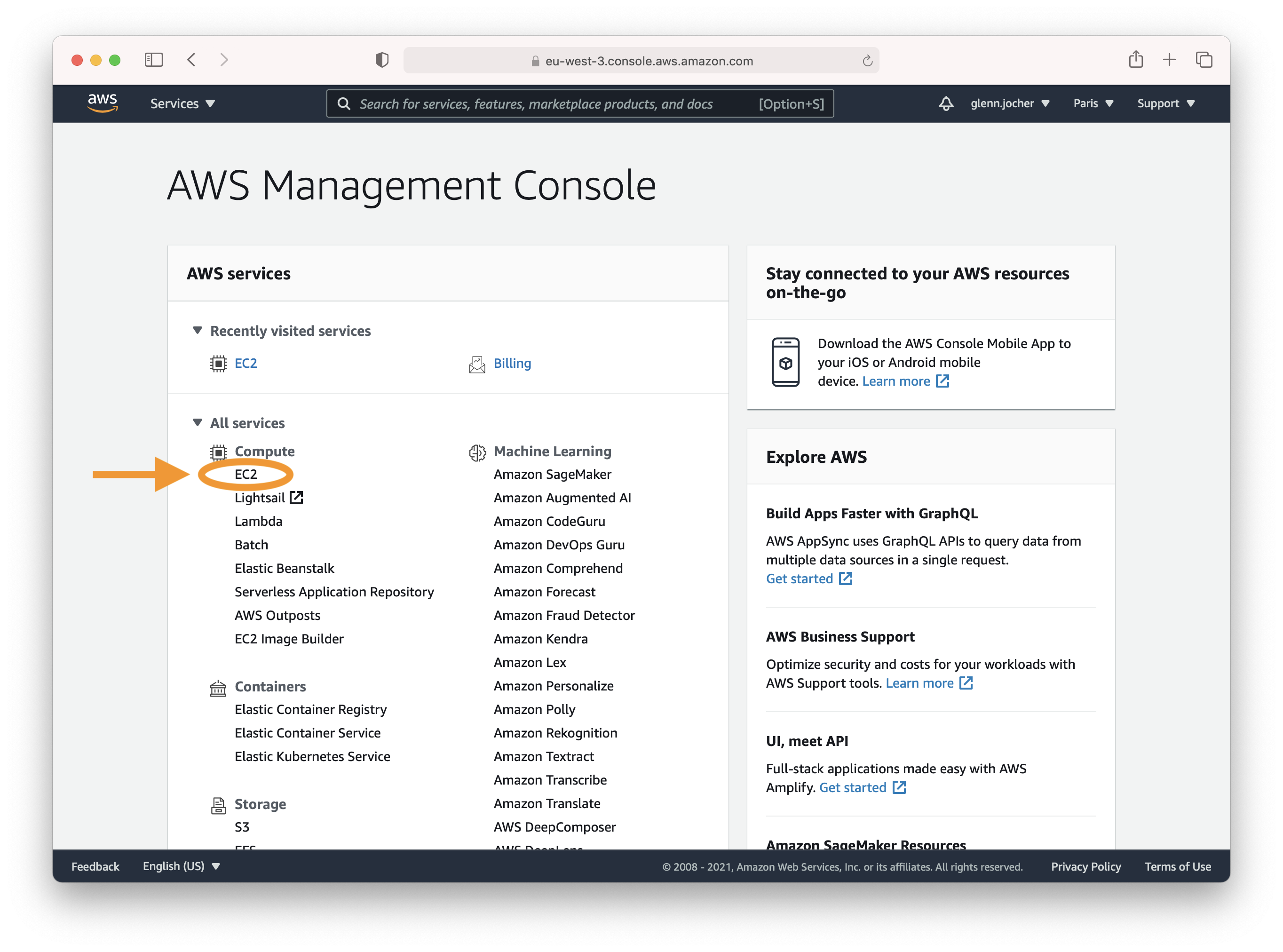
Step 2: Launch Your Instance

In the EC2 dashboard, you'll find the Launch Instance button which is your gateway to creating a new virtual server.

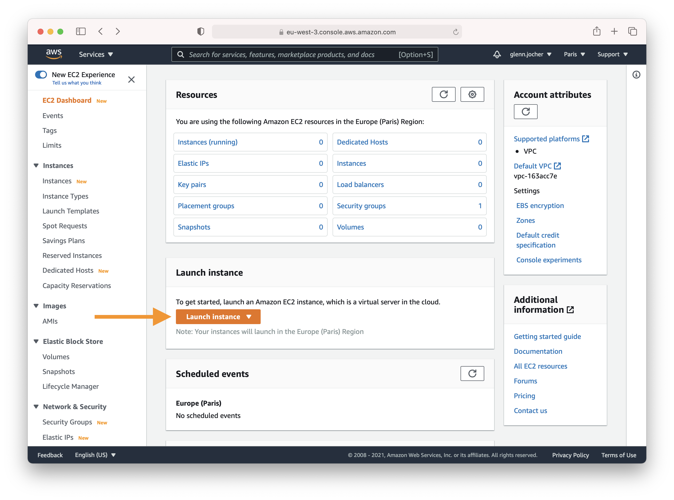
Selecting the Right Amazon Machine Image (AMI)

Here's where you choose the operating system and software stack for your instance. Type 'Deep Learning' into the search field and select the latest Ubuntu-based Deep Learning AMI, unless your needs dictate otherwise. Amazon's Deep Learning AMIs come pre-installed with popular frameworks and GPU drivers to streamline your setup process.

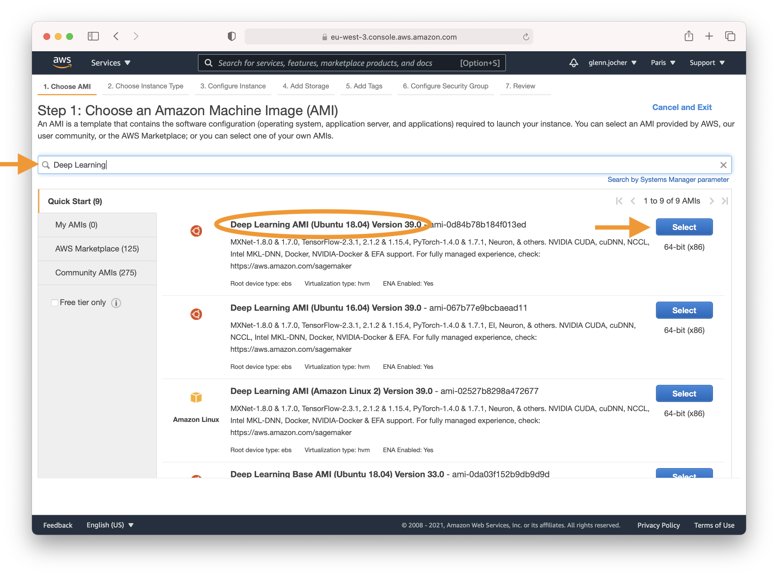
Picking an Instance Type

For deep learning tasks, selecting a GPU instance type is generally recommended as it can vastly accelerate model training. For instance size considerations, remember that the model's memory requirements should never exceed what your instance can provide.

Note: The size of your model should be a factor in selecting an instance. If your model exceeds an instance's available RAM, select a different instance type with enough memory for your application.

For a list of available GPU instance types, visit EC2 Instance Types, specifically under Accelerated Computing.

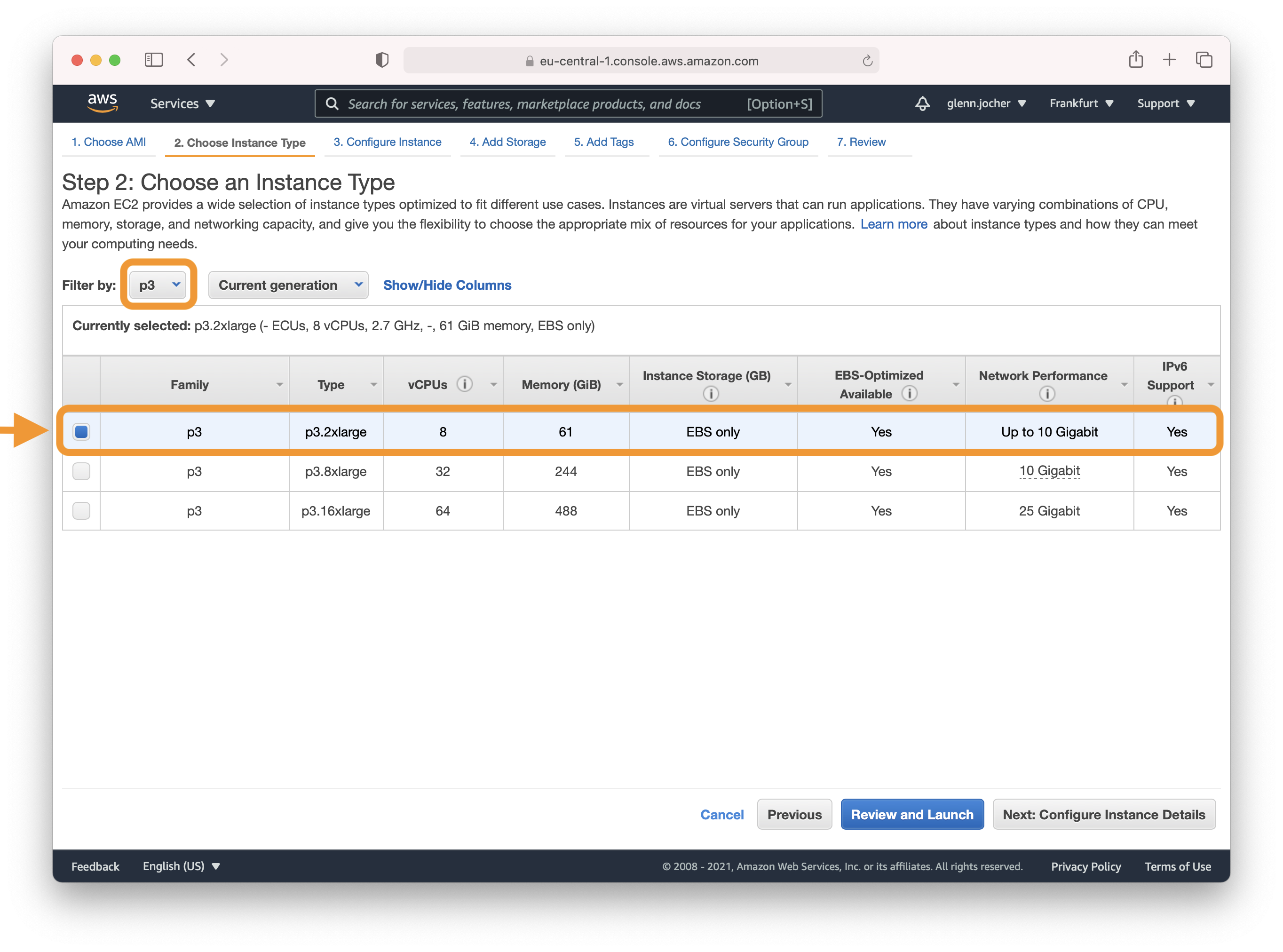
For more information on GPU monitoring and optimization, see GPU Monitoring and Optimization. For pricing, see On-Demand Pricing and Spot Pricing.

Configuring Your Instance

Amazon EC2 Spot Instances offer a cost-effective way to run applications as they allow you to bid for unused capacity at a fraction of the standard cost. For a persistent experience that retains data even when the Spot Instance goes down, opt for a persistent request.

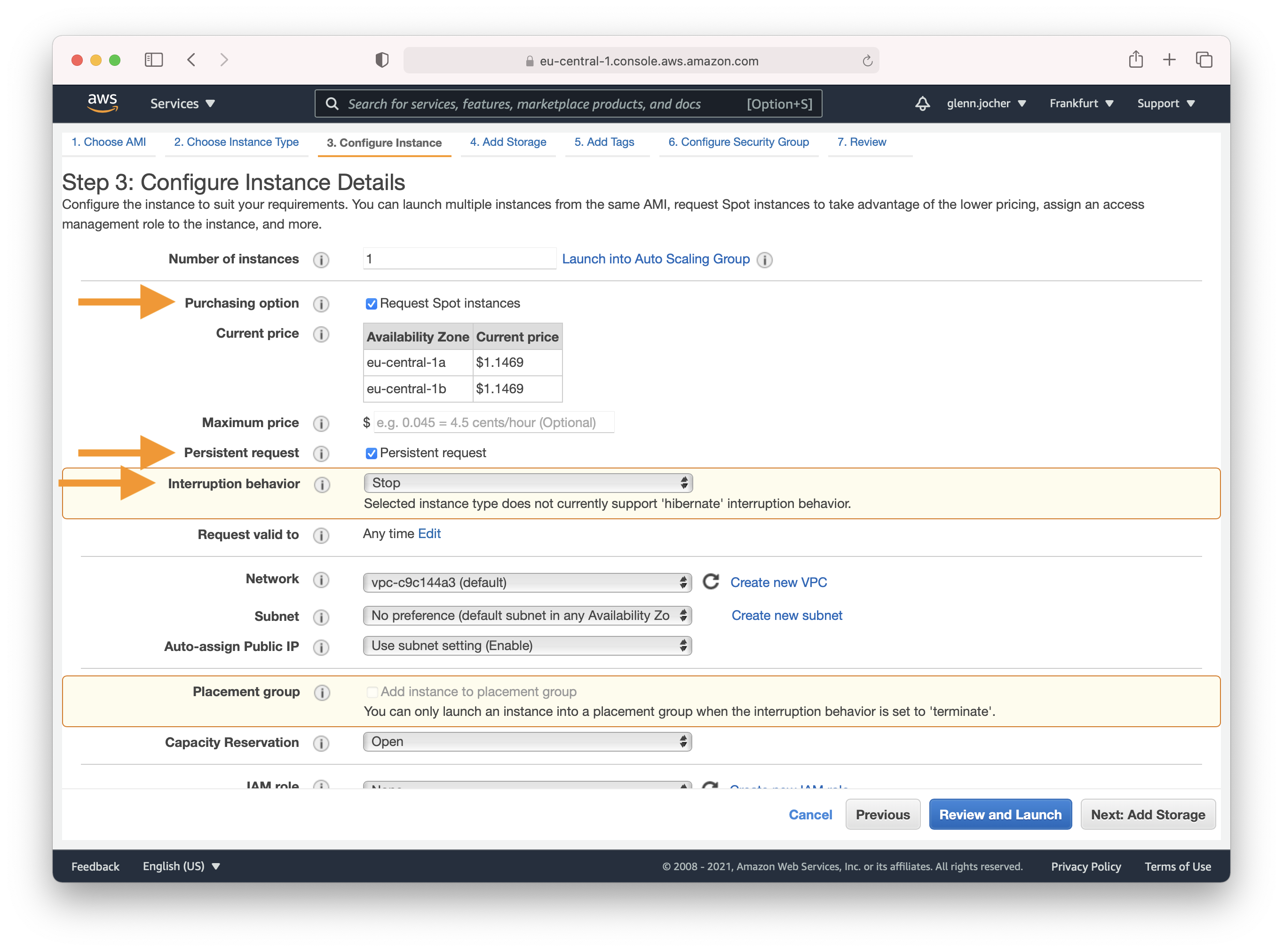
Remember to adjust the rest of your instance settings and security configurations as needed in Steps 4-7 before launching.

Step 3: Connect to Your Instance

Once your instance is running, select its checkbox and click Connect to access the SSH information. Use the displayed SSH command in your preferred terminal to establish a connection to your instance.

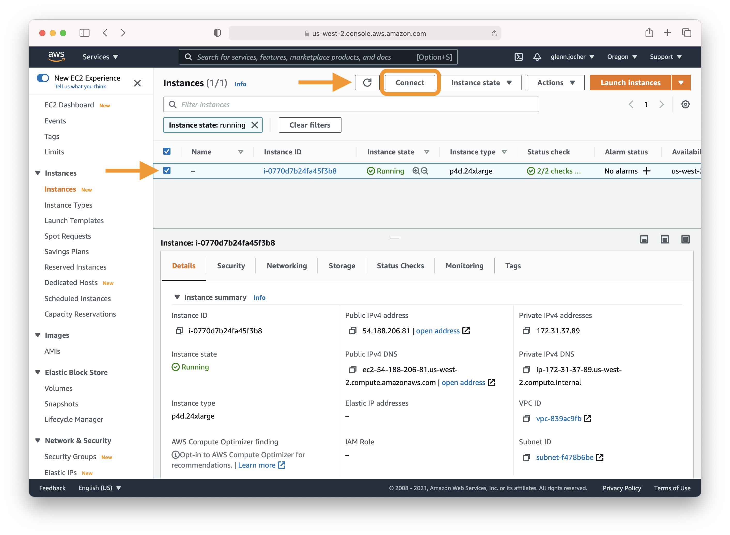
Step 4: Running YOLOv5

Logged into your instance, you're now ready to clone the YOLOv5 repository and install dependencies within a Python 3.8 or later environment. YOLOv5's models and datasets will automatically download from the latest release.

git clone https://github.com/ultralytics/yolov5  # clone repository
cd yolov5
pip install -r requirements.txt  # install dependencies

With your environment set up, you can begin training, validating, performing inference, and exporting your YOLOv5 models:

# Train a model on your data
python train.py

# Validate the trained model for Precision, Recall, and mAP
python val.py --weights yolov5s.pt

# Run inference using the trained model on your images or videos
python detect.py --weights yolov5s.pt --source path/to/images

# Export the trained model to other formats for deployment
python export.py --weights yolov5s.pt --include onnx coreml tflite

Optional Extras

To add more swap memory, which can be a savior for large datasets, run:

sudo fallocate -l 64G /swapfile  # allocate 64GB swap file
sudo chmod 600 /swapfile  # modify permissions
sudo mkswap /swapfile  # set up a Linux swap area
sudo swapon /swapfile  # activate swap file
free -h  # verify swap memory

And that's it! 🎉 You've successfully created an AWS Deep Learning instance and run YOLOv5. Whether you're just starting with object detection or scaling up for production, this setup can help you achieve your machine learning goals. Happy training, validating, and deploying! If you encounter any hiccups along the way, the robust AWS documentation and the active Ultralytics community are here to support you.

---

comments: true
description: Learn how to set up and run YOLOv5 on AzureML. Follow this quickstart guide for easy configuration and model training on an AzureML compute instance.
keywords: YOLOv5, AzureML, machine learning, compute instance, quickstart, model training, virtual environment, Python, AI, deep learning

YOLOv5 🚀 on AzureML

This guide provides a quickstart to use YOLOv5 from an AzureML compute instance.

Note that this guide is a quickstart for quick trials. If you want to unlock the full power AzureML, you can find the documentation to:

• Create a data asset
• Create an AzureML job
• Register a model

Prerequisites

You need an AzureML workspace.

Create a compute instance

From your AzureML workspace, select Compute > Compute instances > New, select the instance with the resources you need.

Open a Terminal

Now from the Notebooks view, open a Terminal and select your compute.

Setup and run YOLOv5

Now you can, create a virtual environment:

conda create --name yolov5env -y
conda activate yolov5env
conda install pip -y

Clone YOLOv5 repository with its submodules:

git clone https://github.com/ultralytics/yolov5
cd yolov5
git submodule update --init --recursive # Note that you might have a message asking you to add your folder as a safe.directory just copy the recommended command

Install the required dependencies:

pip install -r yolov5/requirements.txt
pip install onnx>=1.10.0

Train the YOLOv5 model:

python train.py

Validate the model for Precision, Recall, and mAP

python val.py --weights yolov5s.pt

Run inference on images and videos:

python detect.py --weights yolov5s.pt --source path/to/images

Export models to other formats:

python detect.py --weights yolov5s.pt --source path/to/images

Notes on using a notebook

Note that if you want to run these commands from a Notebook, you need to create a new Kernel and select your new Kernel on the top of your Notebook.

If you create Python cells it will automatically use your custom environment, but if you add bash cells, you will need to run source activate <your-env> on each of these cells to make sure it uses your custom environment.

For example:

%%bash
source activate newenv
python val.py --weights yolov5s.pt