Normal Equation

Normal equation: Method to solve for \(\theta\) analytically.

  相对于Gradient descent，这种方法不需要通过多次的迭代即可直接求得 \(\theta\)，使得Loss Function的值最小。

  下面是\(n+1\)维参数向量使用Normal equation计算 \(\theta \in R^{n+1}\) 的公式：

\[J(\theta_0,\theta_1,\cdots,\theta_m)=\frac{1}{2m}\sum_{i=1}^m(h_\theta(x^{(i)})-y^{(i)})^2 \]

\[\frac{\sigma}{\sigma\theta_j}J(\theta)=0~~~~(\text{for every }j) \]

  Solve for \(\theta_0,\theta_1,\cdots,\theta_m\)
 

Example:

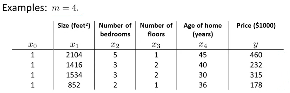
  将表格中的 \(x\) 与 \(y\) 分别写成矩阵的形式：

\[X= \begin{bmatrix} 1 & 2104 & 5 & 1 & 45 \\ 1 & 1416 & 3 & 2 & 40\\ 1 & 1534 & 3 & 2 & 30\\ 1 & 852 & 2 & 1 & 36\\ \end{bmatrix} \]

\[y= \begin{bmatrix} 460 \\ 232 \\ 315 \\ 178 \\ \end{bmatrix} \]

\[\theta=(X^TX)^{-1}X^Ty \]

  此时求得的 \(\theta\) 可以最大限度地减小损失函数的值。
  使用这种方法的时候不需要进行Feature Scaling。
 
|Gradient Descent|Normal Equation|
| ---- | ---- | ---- |
|Need to choose \(\alpha\)|No need to choose \(\alpha\)|
|Needs many iterations|Don't need to iterate|
|\(O(kn^2)\)|\(O(n^3)\)，Need to calculate \((X^TX)^{-1}\)|
|Works well even when \(n\) is large|Slow if \(n\) is very large|
  计算矩阵的逆的时间复杂度为 \(O(n^3)\),所以一般当 \(n>10^5\) 时，会开始使用Gradient Descent，而不是Normal Equation。但是当 \(n\) 的值不是太大的时候，Normal Equation提供了一个计算 \(\theta\) 的好方法。

导致 \(X^TX\)矩阵不可逆的几种可能原因：

• 有冗余的特征（线性相关）
  E.g. \(x_1=size~in~feet^2\)
      \(x_2=size~in~m^2\)
• 过多特征（训练样本数\(m\leq\)特征数\(n\)）
  --删除一些特征或使用正则化