FisherLDA
一 问题描述
• 在 UCI 数据集商的 iris 和 sonar 数据上验证算法的有效性;
• 训练和测试样本有三种方式进行划分:
1)将数据随机分训练样本和测试,多次平均求结果
2)k 折交叉验证
3)留 1 法
二 解决问题的方法
※ 总体概览和声明:
用 fisher 判别分析法训练数据并进行测试。
所用编程语言:Python 所用样本划分方法:K 折交叉验证
所画结果分为两类:iris 数据集的测试样本分布图。
Sonar 数据集经过 3,10,20,30, 40,50,60 维训练后准确度折线图。
1. Fisher 判别分析原理和流程 原理:Fisher linear discriminant analysis(简称 Fisher LDA)是由 FSHER 在 1936 年提出来 的方法。主要思想是将高维样本通过数学变换投影到一维空间中再对其进行分类。如图:
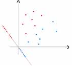
我们通过计算类内离散度矩阵和类间离散度矩阵来判别样本。
假设有N个样本为分别为X=[X1,X2 ……… Xn];用来区分二分类的直线(投影函数)为:

类均值向量为 :

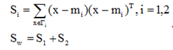
定义各类类内离散度矩阵以及总类内离散度矩阵为:
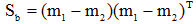
类间离散度矩阵为:
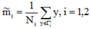
投影后,均值变为:
类内离散度矩阵变为一个值(对于两类问题):
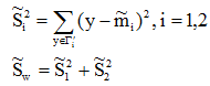
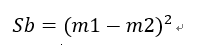
类间离散度矩阵变为两类均值差的平方:
此处m上应该有波浪号
通过化简可以求得Fisher判别准则变为:式1.1
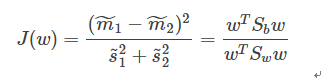
我们的目的就是求使得式1.1最大的投影方向W。因为W幅值的调节不会影响其方向,因此该问题变为一个优化问题:
Max WT*Sb*W(WT是W的转置)
s.t. WT*Sw*W=c(c不等于0)
此时,可引入拉格朗日乘子使该问题转化为一个无约束的优化问题:
L(w,d)= WT*Sb*W -d(WT*Sw*W-c)
通过化简可以得到:W*=Sw求逆*(m1-m2)
代码流程:
1, 取数据,并将其划分为训练集和测试集,此处使用K折交叉验证,通过调参,最终发现7折或8折交叉准确率最大。此处取7折交叉结果作为示例。划分数据的代码存于(util)文件中。对样本标签进行编码。
2, 计算d维的各类的类均值向量Mi
3, 计算类内离散度矩阵和类间离散度矩阵向量
4, 求解矩阵广义特征值问题
5, 为新特征子空间选择线性判别法
6, 将样本转化为新的子空间
7, 计算错误率和准确率
8, 画出训练集的分布关系(只针对iris数据集)
9, 改变样本维度,循环。最后计算所有准确率的平均数(只针对sonar数据集)
10, 画出准确率随着样本维度增加的折线图(只针对sonar数据集)
Iris数据集代码文件:fisherLDA主要程序, util1将数据划分为数据集和训练集的程序, load数据输入转换成矩阵的程序
iris数据集文件:fisherLDA1, util2, load1功能与上面一一对应
这些代码多数来源于github,如有需要请前去搜索,很容易搜到。笔者只进行了一些改动来满足不同的数据。代码环境,pycharm编辑器。win10,64位anaconda,记得将util和load类型的文件保存在Lib当中,python3.6
  1 #!/usr/bin/python3
  2 from load import loader as loader    #作者自己写的程序
  3 from sklearn.preprocessing import LabelEncoder
  4 import numpy as np
  5 from log import log                  #作者自己写的程序
  6 from matplotlib import pyplot as plt
  7 import util1 as util1                #作者自己写的程序
  8
  9 #第一个函数,计算均值向量
 10 def computeMeanVec(X, y, uniqueClass):
 11     """
 12     Step 1: Computing the d-dimensional mean vectors for different class 计算均值向量
 13     """
 14     np.set_printoptions(precision=4)#保留四位小数
 15
 16     mean_vectors = []
 17     for cl in range(1,len(uniqueClass)+1):
 18         mean_vectors.append(np.mean(X[y==cl], axis=0)) #axis = 0:压缩行,对各列求均值,返回 1* n 矩阵
 19         log('Mean Vector class %s: %s\n' %(cl, mean_vectors[cl-1]))#
 20     return mean_vectors
 21
 22 #第二个函数,计算类内离散度矩阵
 23 def computeWithinScatterMatrices(X, y, feature_no, uniqueClass, mean_vectors):
 24     # 2.1 Within-class scatter matrix
 25     S_W = np.zeros((feature_no, feature_no))#初始化矩阵吧
 26     for cl,mv in zip(range(1,len(uniqueClass)+1), mean_vectors):
 27         class_sc_mat = np.zeros((feature_no, feature_no))  # scatter matrix for every class
 28         for row in X[y == cl]:
 29             row, mv = row.reshape(feature_no,1), mv.reshape(feature_no,1)   # make column vectors
 30             class_sc_mat += (row-mv).dot((row-mv).T)
 31         S_W += class_sc_mat                                # sum class scatter matrices
 32     log('within-class Scatter Matrix: {}\n'.format(S_W))
 33
 34     return S_W
 35
 36 #计算类间离散度矩阵
 37 def computeBetweenClassScatterMatrices(X, y, feature_no, mean_vectors):
 38     # 2.2 Between-class scatter matrix
 39     overall_mean = np.mean(X, axis=0)
 40
 41     S_B = np.zeros((feature_no, feature_no))
 42     for i,mean_vec in enumerate(mean_vectors):
 43         n = X[y==i+1,:].shape[0]
 44         mean_vec = mean_vec.reshape(feature_no, 1) # make column vector
 45         overall_mean = overall_mean.reshape(feature_no, 1) # make column vector
 46         S_B += n * (mean_vec - overall_mean).dot((mean_vec - overall_mean).T)
 47     log('between-class Scatter Matrix: {}\n'.format(S_B))
 48
 49     return S_B
 50
 51 def computeEigenDecom(S_W, S_B, feature_no):
 52     """
 53     Step 3: Solving the generalized eigenvalue problem for the matrix S_W^-1 * S_B
 54     求解矩阵 S_W^-1 * S_B 的广义特征值问题
 55     """
 56     m = 10^-6 # add a very small value to the diagonal of your matrix before inversion
 57     #在反演之前向矩阵的对角线增加一个非常小的值
 58     # noinspection PyTypeChecker
 59     eig_vals, eig_vecs = np.linalg.eig(np.linalg.inv(S_W+np.eye(S_W.shape[1])*m).dot(S_B))
 60
 61     for i in range(len(eig_vals)):
 62         eigvec_sc = eig_vecs[:,i].reshape(feature_no, 1)
 63         log('\nEigenvector {}: \n{}'.format(i+1, eigvec_sc.real))
 64         log('Eigenvalue {:}: {:.2e}'.format(i+1, eig_vals[i].real))
 65
 66     for i in range(len(eig_vals)):
 67         eigv = eig_vecs[:,i].reshape(feature_no, 1)
 68         # noinspection PyTypeChecker
 69         np.testing.assert_array_almost_equal(np.linalg.inv(S_W+np.eye(S_W.shape[1])*m).dot(S_B).dot(eigv),
 70                                              eig_vals[i] * eigv,
 71                                              decimal=6, err_msg='', verbose=True)
 72     log('Eigenvalue Decomposition OK')
 73
 74     return eig_vals, eig_vecs
 75
 76 def selectFeature(eig_vals, eig_vecs, feature_no):
 77     """
 78     Step 4: Selecting linear discriminants for the new feature subspace
 79     """
 80     # 4.1. Sorting the eigenvectors by decreasing eigenvalues
 81     # Make a list of (eigenvalue, eigenvector) tuples
 82     eig_pairs = [(np.abs(eig_vals[i]), eig_vecs[:,i]) for i in range(len(eig_vals))]
 83
 84     # Sort the (eigenvalue, eigenvector) tuples from high to low by the value of eigenvalue
 85     eig_pairs = sorted(eig_pairs, key=lambda k: k[0], reverse=True)
 86
 87     log('Eigenvalues in decreasing order:\n')
 88     for i in eig_pairs:
 89         log(i[0])
 90
 91     log('Variance explained:\n')
 92     eigv_sum = sum(eig_vals)
 93     for i,j in enumerate(eig_pairs):
 94         log('eigenvalue {0:}: {1:.2%}'.format(i+1, (j[0]/eigv_sum).real))
 95
 96     # 4.2. Choosing k eigenvectors with the largest eigenvalues - here I choose the first two eigenvalues
 97     W = np.hstack((eig_pairs[0][1].reshape(feature_no, 1), eig_pairs[1][1].reshape(feature_no, 1)))
 98     log('Matrix W: \n{}'.format(W.real))
 99
100     return W
101
102 def transformToNewSpace(X, W, sample_no, mean_vectors, uniqueClass):
103     """
104     Step 5: Transforming the samples onto the new subspace
105     """
106     X_trans = X.dot(W)
107     mean_vecs_trans = []
108     for i in range(len(uniqueClass)):
109         mean_vecs_trans.append(mean_vectors[i].dot(W))
110
111     #assert X_trans.shape == (sample_no,2), "The matrix is not size of (sample number, 2) dimensional."
112
113     return X_trans, mean_vecs_trans
114
115 def computeErrorRate(X_trans, mean_vecs_trans, y):
116     """
117     Compute the error rate
118     """
119
120     """
121     Project to the second largest eigenvalue
122     """
123     uniqueClass = np.unique(y)
124     threshold = 0
125     for i in range(len(uniqueClass)):
126         threshold += mean_vecs_trans[i][1]
127     threshold /= len(uniqueClass)
128     log("threshold: {}".format(threshold))
129
130     errors = 0
131     for (i,cl) in enumerate(uniqueClass):
132         label = cl
133         tmp = X_trans[y==label, 1]
134         # compute the error numbers for class i
135         num = len(tmp[tmp<threshold]) if mean_vecs_trans[i][1] > threshold else len(tmp[tmp>=threshold])
136         log("error rate in class {} = {}".format(i, num*1.0/len(tmp)))
137         errors += num
138
139     errorRate = errors*1.0/X_trans.shape[0]
140     log("Error rate for the second largest eigenvalue = {}".format(errorRate))
141     log("Accuracy for the second largest eigenvalue = {}".format(1-errorRate))
142
143
144     """
145     Project to the largest eigenvalue - and return
146     """
147     uniqueClass = np.unique(y)
148     threshold = 0
149     for i in range(len(uniqueClass)):
150         threshold += mean_vecs_trans[i][0]
151     threshold /= len(uniqueClass)
152     log("threshold: {}".format(threshold))
153
154     errors = 0
155     for (i,cl) in enumerate(uniqueClass):
156         label = cl
157         tmp = X_trans[y==label, 0]
158         # compute the error numbers for class i
159         num = len(tmp[tmp<threshold]) if mean_vecs_trans[i][0] > threshold else len(tmp[tmp>=threshold])
160         log("error rate in class {} = {}".format(i, num*1.0/len(tmp)))
161         errors += num
162
163     errorRate = errors*1.0/X_trans.shape[0]
164     log("Error rate = {}".format(errorRate))
165     log("Accuracy = {}".format(1-errorRate))
166
167     return 1-errorRate, threshold
168
169
170
171
172 def plot_step_lda(X_trans, y, label_dict, uniqueClass, dataset, threshold):
173
174     ax = plt.subplot(111)
175     for label,marker,color in zip(range(1, len(uniqueClass)+1),('^', 's','d'),('blue', 'red','green')):
176         plt.scatter(x=X_trans[:,0].real[y == label],
177                     y=X_trans[:,1].real[y == label],
178                     marker=marker,
179                     color=color,
180                     alpha=0.5,
181                     label=label_dict[label]
182                     )
183
184     plt.xlabel('LDA1')
185     plt.ylabel('LDA2')
186
187     leg = plt.legend(loc='upper right', fancybox=True)
188     #loc 图例所有figure位置,右上。 fancybox控制是否应在构成图例背景的FancyBboxPatch周围启用圆边
189     leg.get_frame().set_alpha(0.5)
190     plt.title('Fisher LDA: {} data projection onto the first 2 linear discriminants'.format(dataset))
191
192     # plot the the threshold line  绘出分界线
193     [bottom, up] = ax.get_ylim()
194     #plt.axvline(x=threshold.real, ymin=bottom, ymax=0.3, linewidth=2, color='k', linestyle='--')
195     plt.axvline(threshold.real, linewidth=2, color='g')
196
197     # hide axis ticks
198     plt.tick_params(axis="both", which="both", bottom="off", top="off",
199             labelbottom="on", left="off", right="off", labelleft="on")
200
201     # remove axis spines
202     ax.spines["top"].set_visible(False)
203     ax.spines["right"].set_visible(False)
204     ax.spines["bottom"].set_visible(False)
205     ax.spines["left"].set_visible(False)
206
207     plt.grid()
208     #plt.tight_layout
209     plt.show()
210
211 def mainFisherLDAtest(dataset='iris', alpha=0.5):  #def mainFisherLDAtest(dataset='sonar', alpha=0.5):
212     # load data
213     path = dataset + '/' + dataset + '.data'
214     load = loader(path)#取数据
215     [X, y] = load.load()
216     # noinspection PyUnresolvedReferences
217     [X, y, testX, testY] = util1.divide(X, y, alpha)#训练集和训练集标签,测试集和测试集标签
218     X = np.array(X) #数组
219     testX = np.array(testX)#测试集
220
221     feature_no = X.shape[1] # define the dimension读取矩阵的维度,返回列数也就是样本维度
222     print(feature_no)
223     sample_no = X.shape[0] # define the sample number返回行数也就是样本个数
224
225     # preprocessing
226     enc = LabelEncoder()
227     label_encoder = enc.fit(y)#对Y进行编码
228
229
230     y = label_encoder.transform(y) + 1#将Y变成正数
231     print(y)
232     testY = label_encoder.transform(testY) + 1#与上文一样
233     # noinspection PyTypeChecker
234     uniqueClass = np.unique(y) # define how many class in the outputs确定有几类输出
235     label_dict = {}   # define the label name
236     for i in range(1, len(uniqueClass)+1):
237         label_dict[i] = "Class"+str(i)
238     log(label_dict)       #打印类别
239
240     # Step 1: Computing the d-dimensional mean vectors for different class
241     mean_vectors = computeMeanVec(X, y, uniqueClass)
242
243
244     # Step 2: Computing the Scatter Matrices
245     S_W = computeWithinScatterMatrices(X, y, feature_no, uniqueClass, mean_vectors)
246     S_B = computeBetweenClassScatterMatrices(X, y, feature_no, mean_vectors)
247
248     # Step 3: Solving the generalized eigenvalue problem for the matrix S_W^-1 * S_B
249     eig_vals, eig_vecs = computeEigenDecom(S_W, S_B, feature_no)
250
251     # Step 4: Selecting linear discriminants for the new feature subspace为新特征子空间选择线性判别法
252     W = selectFeature(eig_vals, eig_vecs, feature_no)
253
254     # Step 5: Transforming the samples onto the new subspace将样本转化为新的子空间
255     X_trans, mean_vecs_trans = transformToNewSpace(testX, W, sample_no, mean_vectors, uniqueClass)
256
257
258     # Step 6: compute error rate
259     accuracy, threshold = computeErrorRate(X_trans, mean_vecs_trans, testY)
260
261
262     # plot
263     plot_step_lda(X_trans, testY, label_dict, uniqueClass, dataset, threshold)
264     #原文这句话被注释了plot_step_lda(X_trans, testY, label_dict, uniqueClass, dataset, threshold)
265
266     return accuracy
267
268
269
270
271 if __name__ == "__main__":
272     dataset = ['ionosphere', 'iris']  # choose the dataset
273     alpha = 0.5  # choose the train data percentage
274     accuracy = mainFisherLDAtest(dataset[1], alpha)
275     print(accuracy)
iris数据导入代码和分割为训练集和测试集代码
 1 import pandas as pd
 2
 3
 4
 5 class loader(object):
 6
 7
 8
 9     def __init__(self,file_name, split_token = ','):#def __init__(self,file_name , split_token = ','):
10
11         self.file_name = 'iris/iris.data'
12
13         self.split_token = split_token
14
15
16
17     def load(self):
18
19         df = pd.io.parsers.read_csv(
20
21             filepath_or_buffer='请在此处写上自己数据的本地路径', #  原文 filepath_or_buffer = self.file_name,笔者用的windows,在路径中用了反斜杠
22
23                             header = None,
24
25                             sep = self.split_token)     #原文 sep = self.split_token)
26
27
28         print(df)
29         print(df.shape[1])
30         self.dimension = df.shape[1]-1
31         print(self.dimension)
32
33         df.columns = list(range(self.dimension)) + ['label']     #原文df.columns = range(self.dimension) + ['label']
34         print(df.columns)
35         df.dropna(how = 'all', inplace = True) # to drop the empty line at file-end 滤除缺失数据
36
37         df.tail() #查看低端数据
38
39
40
41         self.X = df[list(range(self.dimension))].values           # 原文self.X = df[range(self.dimension)].values
42
43         self.Y = df['label'].values
44
45         distinct_label = list(set(self.Y))        #创建分类标签列表
46
47
48
49         if len(distinct_label) != 3:           #原文 if len(distinct_label) != 2:
50
51             raise Exception('Three Labels Required\n','Label Sets:\n',distinct_label)
52             #原文 raise Exception('Two Labels Required\n','Label Sets:\n',distinct_label)
53             #raise Exception是一个函数,用于线程出现异常时抛出错误
54
55
56         self.Y = list(map(lambda x: {distinct_label[0]:1, distinct_label[1]:2,distinct_label[2]:3}[x], self.Y))
57         #原文 self.Y = map(lambda x: {distinct_label[0]: 1, distinct_label[1]: -1}[x], self.Y)
58         print(self.Y)
59
60         return [self.X, self.Y]
61
62
63
64 if __name__ == "__main__":
65
66     loader = loader('iris/iris.data')        #原文 loader = loader('ionosphere/ionosphere.data')
67
68     [X, y] = loader.load()
69
70     print (X.shape)#X是整个数据的大小,Y是标签,共有三个标签
  1 import random
  2
  3 import math
  4
  5 import numpy as np
  6
  7 #将数据分为训练集和数据集
  8
  9 def divide(dataX, dataY, alpha):#x是数据,y是标签
 10
 11     [positiveX, negativeX,X2] = split(dataX, dataY)#分出三类
 12
 13     posNum1 = int(len(positiveX) * alpha)  # alpha=0.5
 14
 15     negNum1 = int(len(negativeX) * alpha)
 16
 17     X2Num1 = int(len(X2) * alpha)
 18
 19     posNum2 = len(positiveX) - posNum1  # 将第一类,第二类,第三类都平均分为两份,一份测试集,一份训练集,这里采用九折交叉
 20
 21     negNum2 = len(negativeX) - negNum1
 22
 23     X2Num2 = len(X2) - X2Num1
 24
 25
 26
 27     posOrder = np.random.permutation(len(positiveX))#分别给两类标上序号
 28
 29     negOrder = np.random.permutation(len(negativeX))
 30
 31     X2Order = np.random.permutation(len(X2))
 32
 33     dataX1 = []#训练集数据
 34
 35     dataY1 = []#训练集标签
 36
 37     dataX2 = []#测试集数据
 38
 39     dataY2 = []#测试集标签
 40
 41
 42
 43
 44     for i in range(posNum1):                            #原文是for i in xrange(posNum1):但是xrange只能用于python2.x,以下全部替换了
 45
 46         dataX1.append(positiveX[posOrder[i]])
 47
 48         dataY1.append(1)
 49
 50     for i in range(posNum2):
 51
 52         dataX2.append(positiveX[posOrder[i + posNum1]])
 53
 54         dataY2.append(1)
 55
 56     for i in range(negNum1):
 57
 58         dataX1.append(negativeX[negOrder[i]])
 59
 60         dataY1.append(-1)
 61
 62     for i in range(negNum2):
 63
 64         dataX2.append(negativeX[negOrder[i + negNum1]])
 65
 66         dataY2.append(-1)
 67     for i in range(X2Num1):
 68
 69         dataX1.append(X2[X2Order[i]])
 70
 71         dataY1.append(2)
 72
 73     for i in range(X2Num2):
 74
 75         dataX2.append(X2[X2Order[i + negNum1]])
 76
 77         dataY2.append(2)
 78
 79
 80
 81     return [dataX1, dataY1, dataX2, dataY2]#返回的是平分的两类数据,x 为数据,y是标签
 82
 83
 84
 85 def resample(dataX, dataY):
 86
 87     '''
 88
 89     sample an equivalent size dataset uniformly from the original one从原始样本中均匀地采样等效大小的数据集
 90
 91     '''
 92
 93     instances = len(dataX)
 94
 95
 96
 97     sampleX = []
 98
 99     sampleY = []
100
101
102
103     for i in range(instances):
104
105         chosen = random.randint(0, instances-1)
106
107         sampleX.append(dataX[chosen])
108
109         sampleY.append(dataY[chosen])
110
111
112
113     return [sampleX, sampleY]
114
115
116
117 def split(dataX, dataY):
118
119     '''
120
121     divide the whole dataset into positive and negative ones 把整个数据集分为正数和负数
122
123     '''
124
125     instances = len(dataX)
126
127     positiveX = []
128
129     negativeX = []
130
131     X2=[]
132
133     for i in range(instances):
134
135         if dataY[i] == 1:
136
137             positiveX.append(dataX[i])
138
139         elif dataY[i] == 2 :
140
141             negativeX.append(dataX[i])
142
143         else :
144
145             X2.append(dataX[i])
146
147
148
149     return [positiveX, negativeX,X2]
150
151
152
153 def F_norm(matrix):
154
155     '''
156
157     calculate the Frobenius norm of a matrix i.e |vec(A)|_2   计算矩阵的Frobenius范数,即VEC(A)2
158
159     '''
160
161     squared = map(lambda x: x**2, matrix)
162
163     squared_sum = np.sum(squared)
164
165     return math.sqrt(squared_sum)
166
167
168
169 def M_norm(matrix, vector):
170
171     '''
172
173     calculate the M-norm of a matrix i.e \sqrt{v.T * M * v}   计算矩阵的m范数,即\sqrt{v.t*m *v}。
174
175     '''
176
177     squared = np.dot(vector.T, np.dot(matrix, vector))
178
179     return math.sqrt(squared[0][0])
sonar代码。功能同上顺序
  1 #!/usr/bin/python3
  2 from load1 import loader as loader    #作者自己写的程序
  3 from sklearn.preprocessing import LabelEncoder
  4 import numpy as np
  5 from log import log                  #作者自己写的程序
  6 from matplotlib import pyplot as plt
  7 import util2 as util2                #作者自己写的程序
  8
  9 #第一个函数,计算均值向量
 10 def computeMeanVec(X, y, uniqueClass):
 11     """
 12     Step 1: Computing the d-dimensional mean vectors for different class 计算均值向量
 13     """
 14     np.set_printoptions(precision=4)#保留四位小数
 15
 16     mean_vectors = []
 17     for cl in range(1,len(uniqueClass)+1):
 18         mean_vectors.append(np.mean(X[y==cl], axis=0)) #axis = 0:压缩行,对各列求均值,返回 1* n 矩阵
 19         log('Mean Vector class %s: %s\n' %(cl, mean_vectors[cl-1]))#
 20     return mean_vectors
 21
 22 #第二个函数,计算类内离散度矩阵
 23 def computeWithinScatterMatrices(X, y, feature_no, uniqueClass, mean_vectors):
 24     # 2.1 Within-class scatter matrix
 25     S_W = np.zeros((feature_no, feature_no))#初始化矩阵吧
 26     for cl,mv in zip(range(1,len(uniqueClass)+1), mean_vectors):
 27         class_sc_mat = np.zeros((feature_no, feature_no))  # scatter matrix for every class
 28         for row in X[y == cl]:
 29             row, mv = row.reshape(feature_no,1), mv.reshape(feature_no,1)   # make column vectors
 30             class_sc_mat += (row-mv).dot((row-mv).T)
 31         S_W += class_sc_mat                                # sum class scatter matrices
 32     log('within-class Scatter Matrix: {}\n'.format(S_W))
 33
 34     return S_W
 35
 36 #计算类间离散度矩阵
 37 def computeBetweenClassScatterMatrices(X, y, feature_no, mean_vectors):
 38     # 2.2 Between-class scatter matrix
 39     overall_mean = np.mean(X, axis=0)
 40
 41     S_B = np.zeros((feature_no, feature_no))
 42     for i,mean_vec in enumerate(mean_vectors):
 43         n = X[y==i+1,:].shape[0]
 44         mean_vec = mean_vec.reshape(feature_no, 1) # make column vector
 45         overall_mean = overall_mean.reshape(feature_no, 1) # make column vector
 46         S_B += n * (mean_vec - overall_mean).dot((mean_vec - overall_mean).T)
 47     log('between-class Scatter Matrix: {}\n'.format(S_B))
 48
 49     return S_B
 50
 51 def computeEigenDecom(S_W, S_B, feature_no):
 52     """
 53     Step 3: Solving the generalized eigenvalue problem for the matrix S_W^-1 * S_B
 54     求解矩阵 S_W^-1 * S_B 的广义特征值问题
 55     """
 56     m = 10^-6 # add a very small value to the diagonal of your matrix before inversion
 57     #在反演之前向矩阵的对角线增加一个非常小的值
 58     # noinspection PyTypeChecker
 59     eig_vals, eig_vecs = np.linalg.eig(np.linalg.inv(S_W+np.eye(S_W.shape[1])*m).dot(S_B))
 60
 61     for i in range(len(eig_vals)):
 62         eigvec_sc = eig_vecs[:,i].reshape(feature_no, 1)
 63         log('\nEigenvector {}: \n{}'.format(i+1, eigvec_sc.real))
 64         log('Eigenvalue {:}: {:.2e}'.format(i+1, eig_vals[i].real))
 65
 66     for i in range(len(eig_vals)):
 67         eigv = eig_vecs[:,i].reshape(feature_no, 1)
 68         # noinspection PyTypeChecker
 69         np.testing.assert_array_almost_equal(np.linalg.inv(S_W+np.eye(S_W.shape[1])*m).dot(S_B).dot(eigv),
 70                                              eig_vals[i] * eigv,
 71                                              decimal=6, err_msg='', verbose=True)
 72     log('Eigenvalue Decomposition OK')
 73
 74     return eig_vals, eig_vecs
 75
 76 def selectFeature(eig_vals, eig_vecs, feature_no):
 77     """
 78     Step 4: Selecting linear discriminants for the new feature subspace
 79     """
 80     # 4.1. Sorting the eigenvectors by decreasing eigenvalues
 81     # Make a list of (eigenvalue, eigenvector) tuples
 82     eig_pairs = [(np.abs(eig_vals[i]), eig_vecs[:,i]) for i in range(len(eig_vals))]
 83
 84     # Sort the (eigenvalue, eigenvector) tuples from high to low by the value of eigenvalue
 85     eig_pairs = sorted(eig_pairs, key=lambda k: k[0], reverse=True)
 86
 87     log('Eigenvalues in decreasing order:\n')
 88     for i in eig_pairs:
 89         log(i[0])
 90
 91     log('Variance explained:\n')
 92     eigv_sum = sum(eig_vals)
 93     for i,j in enumerate(eig_pairs):
 94         log('eigenvalue {0:}: {1:.2%}'.format(i+1, (j[0]/eigv_sum).real))
 95
 96     # 4.2. Choosing k eigenvectors with the largest eigenvalues - here I choose the first two eigenvalues
 97     W = np.hstack((eig_pairs[0][1].reshape(feature_no, 1), eig_pairs[1][1].reshape(feature_no, 1)))
 98     log('Matrix W: \n{}'.format(W.real))
 99
100     return W
101
102 def transformToNewSpace(X, W, sample_no, mean_vectors, uniqueClass):
103     """
104     Step 5: Transforming the samples onto the new subspace
105     """
106     X_trans = X.dot(W)
107     mean_vecs_trans = []
108     for i in range(len(uniqueClass)):
109         mean_vecs_trans.append(mean_vectors[i].dot(W))
110
111     #assert X_trans.shape == (sample_no,2), "The matrix is not size of (sample number, 2) dimensional."
112
113     return X_trans, mean_vecs_trans
114
115 def computeErrorRate(X_trans, mean_vecs_trans, y):
116     """
117     Compute the error rate
118     """
119
120     """
121     Project to the second largest eigenvalue
122     """
123     uniqueClass = np.unique(y)
124     threshold = 0
125     for i in range(len(uniqueClass)):
126         threshold += mean_vecs_trans[i][1]
127     threshold /= len(uniqueClass)
128     log("threshold: {}".format(threshold))
129
130     errors = 0
131     for (i,cl) in enumerate(uniqueClass):
132         label = cl
133         tmp = X_trans[y==label, 1]
134         # compute the error numbers for class i
135         num = len(tmp[tmp<threshold]) if mean_vecs_trans[i][1] > threshold else len(tmp[tmp>=threshold])
136         log("error rate in class {} = {}".format(i, num*1.0/len(tmp)))
137         errors += num
138
139     errorRate = errors*1.0/X_trans.shape[0]
140     log("Error rate for the second largest eigenvalue = {}".format(errorRate))
141     log("Accuracy for the second largest eigenvalue = {}".format(1-errorRate))
142
143
144     """
145     Project to the largest eigenvalue - and return
146     """
147     uniqueClass = np.unique(y)
148     threshold = 0
149     for i in range(len(uniqueClass)):
150         threshold += mean_vecs_trans[i][0]
151     threshold /= len(uniqueClass)
152     log("threshold: {}".format(threshold))
153
154     errors = 0
155     for (i,cl) in enumerate(uniqueClass):
156         label = cl
157         tmp = X_trans[y==label, 0]
158         # compute the error numbers for class i
159         num = len(tmp[tmp<threshold]) if mean_vecs_trans[i][0] > threshold else len(tmp[tmp>=threshold])
160         log("error rate in class {} = {}".format(i, num*1.0/len(tmp)))
161         errors += num
162
163     errorRate = errors*1.0/X_trans.shape[0]
164     log("Error rate = {}".format(errorRate))
165     log("Accuracy = {}".format(1-errorRate))
166
167     return 1-errorRate, threshold
168
169
170
171
172 def plot_step_lda(X_trans, y, label_dict, uniqueClass, dataset, threshold):
173
174     ax = plt.subplot(111)
175     for label,marker,color in zip(range(1, len(uniqueClass)+1),('^', 's','d'),('blue', 'red','green')):
176         plt.scatter(x=X_trans[:,0].real[y == label], #X[:,0]就是取所有行的第0个数据, X[:,1] 就是取所有行的第1个数据
177                     y=X_trans[:,1].real[y == label],
178                     marker=marker,
179                     color=color,
180                     alpha=0.5,
181                     label=label_dict[label]
182                     )
183
184     plt.xlabel('LDA1')
185     plt.ylabel('LDA2')
186
187     leg = plt.legend(loc='upper right', fancybox=True)
188     #loc 图例所有figure位置,右上。 fancybox控制是否应在构成图例背景的FancyBboxPatch周围启用圆边
189     leg.get_frame().set_alpha(0.5)
190     plt.title('Fisher LDA: {} data projection onto the first 2 linear discriminants'.format(dataset))
191
192     # plot the the threshold line  绘出分界线
193     [bottom, up] = ax.get_ylim()
194     #plt.axvline(x=threshold.real, ymin=bottom, ymax=0.3, linewidth=2, color='k', linestyle='--')
195     plt.axvline(threshold.real, linewidth=2, color='g')
196
197     # hide axis ticks
198     plt.tick_params(axis="both", which="both", bottom="off", top="off",
199             labelbottom="on", left="off", right="off", labelleft="on")
200
201     # remove axis spines
202     ax.spines["top"].set_visible(False)
203     ax.spines["right"].set_visible(False)
204     ax.spines["bottom"].set_visible(False)
205     ax.spines["left"].set_visible(False)
206
207     plt.grid()
208     #plt.tight_layout
209     plt.show()
210     #第二个图
211 def plot_step_lda2(accuracys):
212     ax = plt.subplot(111)
213     plt.xlabel('Demention')
214     plt.ylabel('Accuracy')
215
216     leg = plt.legend(loc='upper right', fancybox=True)
217     # loc 图例所有figure位置,右上。 fancybox控制是否应在构成图例背景的FancyBboxPatch周围启用圆边
218     leg.get_frame().set_alpha(0.5)
219     plt.title('Fisher LDA: {} data projection onto the first 2 linear discriminants'.format(dataset))
220     plt.axis([0, 60, 0, 1])
221     x=[3, 10, 20, 30, 40, 50, 60]
222     y=accuracys
223     plt.plot(x,y,linewidth=1,color='b')
224     plt.show()
225
226 def mainFisherLDAtest(dataset='sonar', alpha=0.5):  #def mainFisherLDAtest(dataset='sonar', alpha=0.5):
227     # load data
228     path = dataset + '/' + dataset + '.data'
229     load = loader(path)#取数据
230     [X, y] = load.load()
231     [x1,y1]=[X,y]
232     # noinspection PyUnresolvedReferences
233     #改动,进行交叉验证
234     dimension=[3,10,20,30,40,50,60]
235     accuracys=[0,0,0,0,0,0,0]
236     accnumber=0
237     for i in range(7):
238         [X, y]=[x1,y1]
239         j=dimension[i]
240         [X, y, testX, testY] = util2.divide(X, y, alpha,j)#训练集和训练集标签,测试集和测试集标签
241         X = np.array(X) #数组
242         testX = np.array(testX)#测试集
243
244         feature_no = X.shape[1] # define the dimension读取矩阵的维度,返回列数也就是样本维度
245         print(feature_no)
246         sample_no = X.shape[0] # define the sample number返回行数也就是样本个数
247
248     # preprocessing
249         enc = LabelEncoder()
250         label_encoder = enc.fit(y)#对Y进行编码
251
252
253         y = label_encoder.transform(y) + 1#将Y变成正数
254         print(y)
255         testY = label_encoder.transform(testY) + 1#与上文一样
256     # noinspection PyTypeChecker
257         uniqueClass = np.unique(y) # define how many class in the outputs确定有几类输出
258         label_dict = {}   # define the label name
259         for i in range(1, len(uniqueClass)+1):
260             label_dict[i] = "Class"+str(i)
261         log(label_dict)       #打印类别
262
263     # Step 1: Computing the d-dimensional mean vectors for different class
264         mean_vectors = computeMeanVec(X, y, uniqueClass)
265
266
267     # Step 2: Computing the Scatter Matrices
268         S_W = computeWithinScatterMatrices(X, y, feature_no, uniqueClass, mean_vectors)
269         S_B = computeBetweenClassScatterMatrices(X, y, feature_no, mean_vectors)
270
271     # Step 3: Solving the generalized eigenvalue problem for the matrix S_W^-1 * S_B
272         eig_vals, eig_vecs = computeEigenDecom(S_W, S_B, feature_no)
273
274     # Step 4: Selecting linear discriminants for the new feature subspace为新特征子空间选择线性判别法
275         W = selectFeature(eig_vals, eig_vecs, feature_no)
276
277     # Step 5: Transforming the samples onto the new subspace将样本转化为新的子空间
278         X_trans, mean_vecs_trans = transformToNewSpace(testX, W, sample_no, mean_vectors, uniqueClass)
279
280
281     # Step 6: compute error rate
282         accuracy, threshold = computeErrorRate(X_trans, mean_vecs_trans, testY)
283
284
285     # plot
286         plot_step_lda(X_trans, testY, label_dict, uniqueClass, dataset, threshold)
287     #plot_step_lda(X_trans, testY, label_dict, uniqueClass, dataset, threshold)
288         accuracys[accnumber] = accuracy
289         accnumber = accnumber + 1
290     plot_step_lda2(accuracys)
291     accuracy = ( accuracys[0] + accuracys[1] +accuracys[2] + accuracys[3] + accuracys[4] + accuracys[5]+ accuracys[6])/6
292     return accuracy
293
294
295
296
297 if __name__ == "__main__":
298     dataset = ['ionosphere', 'sonar']  # choose the dataset
299     alpha = 0.7 # choose the train data percentage
300     accuracy = mainFisherLDAtest(dataset[1], alpha)
301     print(accuracy)
 1 import pandas as pd
 2
 3
 4
 5 class loader(object):
 6
 7
 8
 9     def __init__(self,file_name, split_token = ','):#def __init__(self,file_name , split_token = ','):
10
11         self.file_name = 'sonar/sonar.data'
12
13         self.split_token = split_token
14
15
16
17     def load(self):
18
19         df = pd.io.parsers.read_csv(
20
21             filepath_or_buffer='请在此处写上自己数据的本地路径', #  原文 filepath_or_buffer = self.file_name,
22
23                             header = None,
24
25                             sep = self.split_token)     #原文 sep = self.split_token)
26
27
28
29
30         self.dimension = df.shape[1]-1
31
32
33         df.columns = list(range(self.dimension)) + ['label']     #原文df.columns = range(self.dimension) + ['label']
34
35         df.dropna(how = 'all', inplace = True) # to drop the empty line at file-end 滤除缺失数据
36
37         df.tail() #查看低端数据
38
39
40
41         self.X = df[list(range(self.dimension))].values           # 原文self.X = df[range(self.dimension)].values
42
43         self.Y = df['label'].values
44
45         distinct_label = list(set(self.Y))        #创建分类标签列表
46
47
48
49         if len(distinct_label) != 2:           #原文 if len(distinct_label) != 2:
50
51             raise Exception('Two Labels Required\n','Label Sets:\n',distinct_label)
52             #原文 raise Exception('Two Labels Required\n','Label Sets:\n',distinct_label)
53             #raise Exception是一个函数,用于线程出现异常时抛出错误
54
55
56         self.Y = list(map(lambda x: {distinct_label[0]:1, distinct_label[1]:-1}[x], self.Y))
57         #原文 self.Y = map(lambda x: {distinct_label[0]: 1, distinct_label[1]: -1}[x], self.Y)
58
59         return [self.X, self.Y]
60
61
62
63 if __name__ == "__main__":
64
65     loader = loader('ionosphere/ionosphere.data')        #原文 loader = loader('ionosphere/ionosphere.data')
66
67     [X, y] = loader.load()
68
69     print (X.shape)#X是整个数据的大小,Y是标签,共有三个标签
import random

import math

import numpy as np

#将数据分为训练集和数据集
#x是数据,y是标签
#divide a dataset into two parts, usually training and testing set
def divide(dataX, dataY, alpha,i):
    print(i)
    d=[]
    for k in range(i):
        d.append(k)

    print(d)
    dataX=dataX[:,d]
    print(dataX)

    [positiveX, negativeX] = split(dataX, dataY)#分出两类
    # alpha=0.5
    posNum1 = int (len(positiveX) * alpha)

    negNum1 = int (len(negativeX) * alpha)

    posNum2 = len(positiveX) - posNum1

    negNum2 = len(negativeX) - negNum1
    # 将第一类,第二类
    posOrder = np.random.permutation(len(positiveX))#分别给两类标上序号

    negOrder = np.random.permutation(len(negativeX))

    dataX1 = []

    dataY1 = []

    dataX2 = []

    dataY2 = []

    for i in range(posNum1):

        dataX1.append(positiveX[posOrder[i]])

        dataY1.append(1)

    for i in range(posNum2):

        dataX2.append(positiveX[posOrder[i + posNum1]])

        dataY2.append(1)

    for i in range(negNum1):

        dataX1.append(negativeX[negOrder[i]])

        dataY1.append(-1)

    for i in range(negNum2):

        dataX2.append(negativeX[negOrder[i + negNum1]])

        dataY2.append(-1)


    return [dataX1, dataY1, dataX2, dataY2]#返回的是平分的两类数据


def resample(dataX, dataY):

    '''

    sample an equivalent size dataset uniformly from the original one从原始样本中均匀地采样等效大小的数据集

    '''

    instances = len(dataX)


    sampleX = []

    sampleY = []


    for i in range(instances):

        chosen = random.randint(0, instances-1)

        sampleX.append(dataX[chosen])

        sampleY.append(dataY[chosen])


    return [sampleX, sampleY]


def split(dataX, dataY):

    '''

    divide the whole dataset into positive and negative ones 把整个数据集分为正数和负数

    '''

    instances = len(dataX)

    positiveX = []

    negativeX = []


    for i in range(instances):

        if dataY[i] == 1:

            positiveX.append(dataX[i])

        else:

            negativeX.append(dataX[i])


    return [positiveX, negativeX]


def F_norm(matrix):

    '''

    calculate the Frobenius norm of a matrix i.e |vec(A)|_2   计算矩阵的Frobenius范数,即VEC(A)2

    '''

    squared = map(lambda x: x**2, matrix)

    squared_sum = np.sum(squared)

    return math.sqrt(squared_sum)


def M_norm(matrix, vector):

    '''

    calculate the M-norm of a matrix i.e \sqrt{v.T * M * v}   计算矩阵的m范数,即\sqrt{v.t*m *v}。

    '''

    squared = np.dot(vector.T, np.dot(matrix, vector))

    return math.sqrt(squared[0][0])
就这些了。

 浙公网安备 33010602011771号