【数值计算方法】非线性方程求根-数值实验
 数值实验python实验
第一题
newton method
非线性方程组的向量函数为:
迭代格式为:
其中\([F'(x,y)]\)为\(F(x,y)\)的Jacobian矩阵:
from formu_lib import *
import numpy as np
from matplotlib import pyplot as plt

def F(x:np.ndarray)->np.ndarray:
    x,y=x[0],x[1]

    f1=(x-2)**2+(y-3+2*x)**2-5
    f2=2*(x-3)**2+(y/3.0)**2-4
    return np.array([f1,f2])

def DF(x:np.ndarray)->np.ndarray:
    x,y=x[0],x[1]
    f11=2*(x-2)+4*(y-3+2*x)
    f12=4*(y-3+2*x)
    f21=4*(x-3)
    f22=(2*y)/9.0
    return np.array([[f11,f12],
                    [f21,f22]])

x0=np.array([0,0])
tol=1e-10
maxiter=100

x,res=NonlinearEquationsNewtonMethod(F,DF,x0,tol,maxiter)
plt.plot(list(range(len(res))),res,label='residual-norm',marker='o')
plt.xlabel('iteration')
plt.ylabel('residual-norm(F(x))')
plt.legend()
plt.title('residual-norm VS iteration')
plt.show()

print(f"results:")
print(f"root:{x},residual-norm:{res[-1]}")
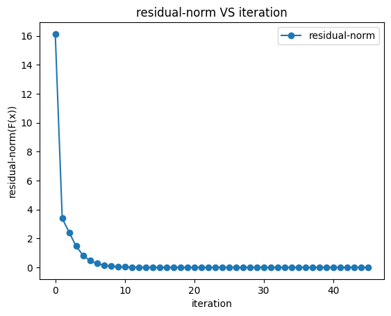
- results:
root:[ 1.7362259 -2.69290744],residual-norm:8.749090341098054e-11
quasi-newton method
拟牛顿法的迭代格式为:
取单位矩阵为B0矩阵,使用秩一修正 (Rank 1 Update) 公式修正B矩阵:
from formu_lib import *
import numpy as np
from matplotlib import pyplot as plt
from numpy.linalg import inv,norm

def F(xs:np.ndarray)->np.ndarray:
    x,y=xs[0],xs[1]

    f1=(x-2)**2+(y-3+2*x)**2-5
    f2=2*(x-3)**2+(y/3.0)**2-4
    return np.array([f1,f2])

x0=np.array([1,1])
B0=np.eye(2)
tol=1e-10
maxiter=100

x,res=NonliearEquationsQuasi_NewtonMethod(F,B0,x0,tol,maxiter)

# 绘图
plt.plot(list(range(len(res))),res,label=f' quasi-newton method Iter,num:{len(res)}',marker='o')
plt.xlabel('iteration')
plt.ylabel('residual-norm(F(x))')
plt.legend()
plt.title('residual-norm VS iteration')
plt.show()

print(f"results:")
print(f"+ quasi-newton method Iter,num:{len(res)},root:{x},residual-norm:{res[-1]}")
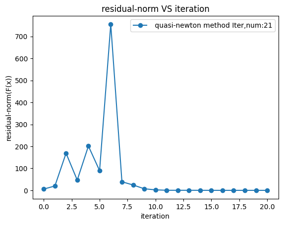
- results of quasi-newton method Iter:
- num:21
- root:[ 4.02873354 -4.1171266 ]
- residual-norm:1.855071568790407e-12
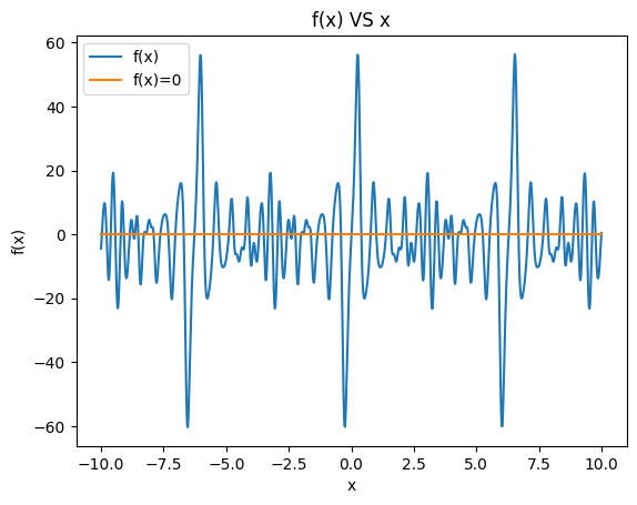
第二题
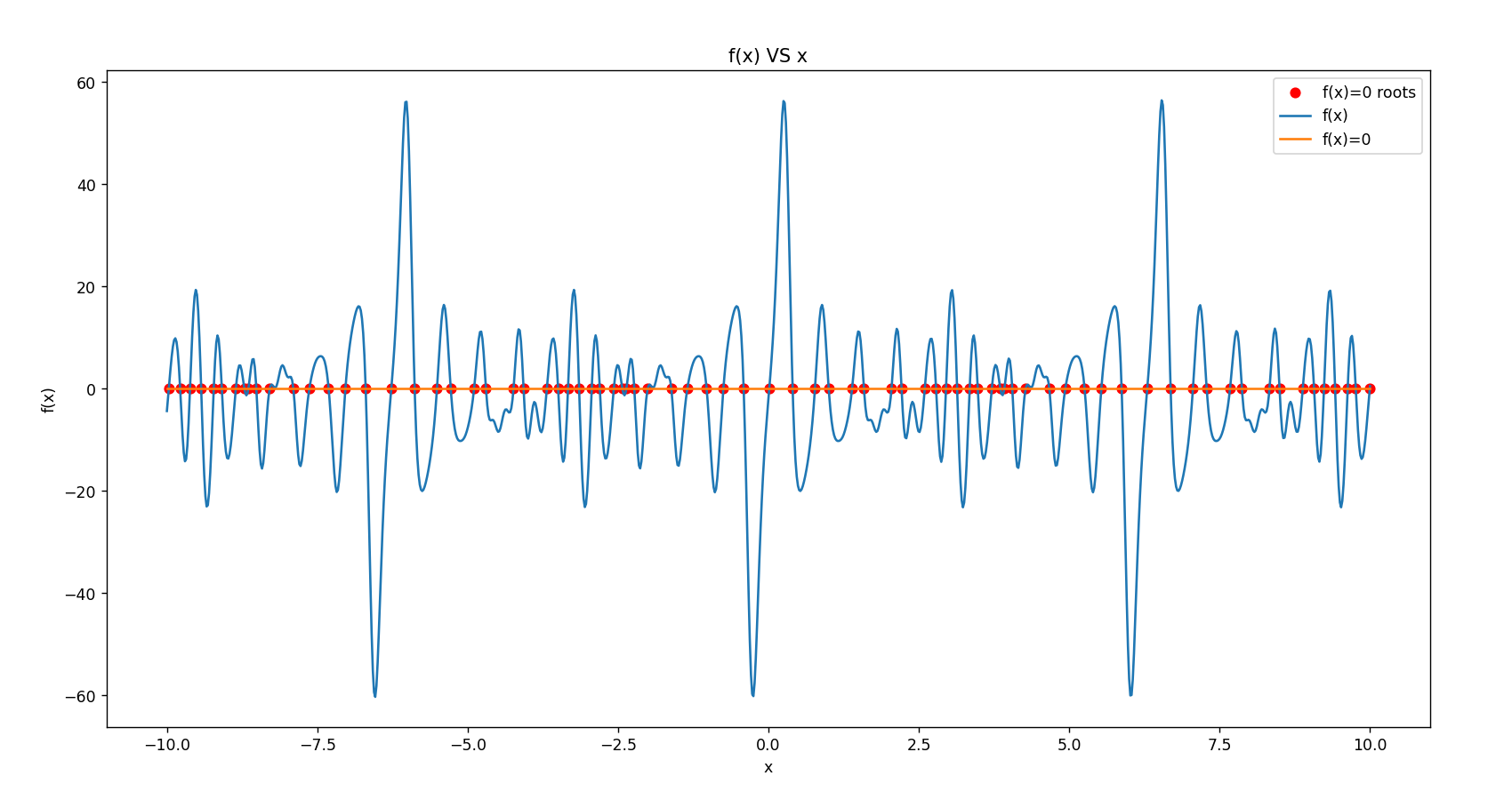
可以使用牛顿法,割线法,二分法,不动点迭代法计算非线性方程组在[-10,10]的根:
原函数的图像为:
原函数图像python code
from formu_lib import *
import numpy as np
from matplotlib import pyplot as plt

def f(x:float)->float:
    def ff(x,k):
        return k*np.exp(-np.cos(k*x))*np.sin(k*x)
    return sum([ff(x,k) for k in range(1,11)])-2

a,b=-10,10
num=1000
x=np.linspace(a,b,num)
y=[f(i) for i in x]

plt.plot(x,y,label='f(x)')
plt.plot([a,b],[0,0],label='f(x)=0')
plt.xlabel('x')
plt.ylabel('f(x)')
plt.legend()
plt.title('f(x) VS x')
plt.show()
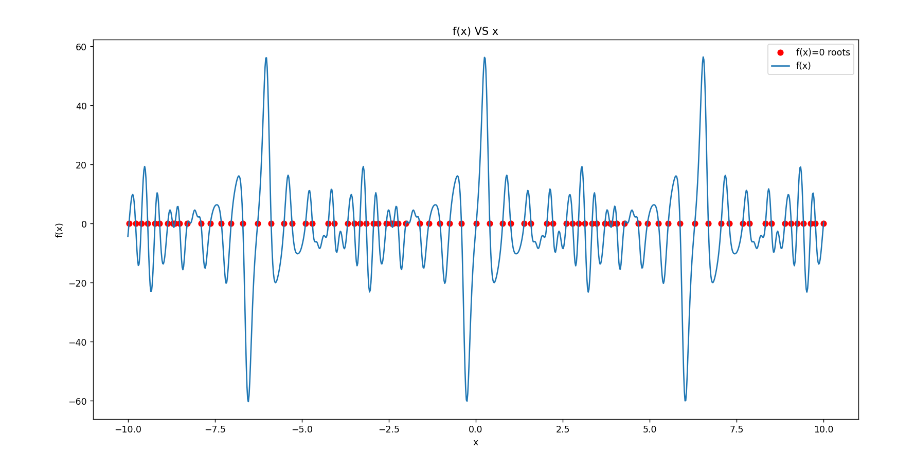
使用复合二分法求根
roots=ComBSMethod(f,a,b,2000,1e-10)
print(f"results:{roots}")
plt.scatter(roots,[f(root)for root in roots],label='f(x)=0 roots',marker='o')
结果:
ComBSMethod time:0.369394 s
复合二分法求根结果
root_1 , val_1 = -9.9674243606 , 误差 = -3.64980e-09
root_2 , val_2 = -9.7797174668 , 误差 = -6.61337e-09
root_3 , val_3 = -9.6149032646 , 误差 = -1.38758e-09
root_4 , val_4 = -9.4302274624 , 误差 = -7.99506e-09
root_5 , val_5 = -9.2207822340 , 误差 = -5.04254e-09
root_6 , val_6 = -9.0871043562 , 误差 = 6.59284e-09
root_7 , val_7 = -8.8530192104 , 误差 = 1.21289e-09
root_8 , val_8 = -8.7125086779 , 误差 = -3.74143e-11
root_9 , val_9 = -8.6442340327 , 误差 = -2.62465e-09
root_10 , val_10 = -8.5133652799 , 误差 = 4.73630e-09
root_11 , val_11 = -8.2899925123 , 误差 = -1.15093e-09
root_12 , val_12 = -7.8981572476 , 误差 = -2.71837e-09
root_13 , val_13 = -7.6307012374 , 误差 = 1.03455e-09
root_14 , val_14 = -7.3115311582 , 误差 = 1.90418e-09
root_15 , val_15 = -7.0320102647 , 误差 = -3.08314e-09
root_16 , val_16 = -6.6955392638 , 误差 = 1.15621e-09
root_17 , val_17 = -6.2691253474 , 误差 = 2.07994e-09
root_18 , val_18 = -5.8813837698 , 误差 = 1.17033e-08
root_19 , val_19 = -5.5099115066 , 误差 = 4.09161e-09
root_20 , val_20 = -5.2816152127 , 误差 = -1.69667e-09
root_21 , val_21 = -4.8929026655 , 误差 = -2.34091e-10
root_22 , val_22 = -4.6958911892 , 误差 = -3.00448e-09
root_23 , val_23 = -4.2373378929 , 误差 = -2.08822e-09
root_24 , val_24 = -4.0708334564 , 误差 = 4.54090e-09
root_25 , val_25 = -3.6842390533 , 误差 = 4.17905e-09
root_26 , val_26 = -3.4965321596 , 误差 = -2.23404e-09
root_27 , val_27 = -3.3317179574 , 误差 = -7.17032e-09
root_28 , val_28 = -3.1470421552 , 误差 = -8.36770e-10
root_29 , val_29 = -2.9375969268 , 误差 = 1.02456e-08
root_30 , val_30 = -2.8039190489 , 误差 = -6.32259e-09
root_31 , val_31 = -2.5698339033 , 误差 = -1.27755e-09
root_32 , val_32 = -2.4293233707 , 误差 = 1.34728e-09
root_33 , val_33 = -2.3610487255 , 误差 = 1.62072e-09
root_34 , val_34 = -2.2301799727 , 误差 = -6.62781e-09
root_35 , val_35 = -2.0068072050 , 误差 = 1.93580e-09
root_36 , val_36 = -1.6149719405 , 误差 = -5.79220e-10
root_37 , val_37 = -1.3475159302 , 误差 = -4.51056e-10
root_38 , val_38 = -1.0283458510 , 误差 = 4.41240e-09
root_39 , val_39 = -0.7488249574 , 误差 = 5.23588e-09
root_40 , val_40 = -0.4123539567 , 误差 = 8.09918e-09
root_41 , val_41 = 0.0140599598 , 误差 = -7.27386e-10
root_42 , val_42 = 0.4018015374 , 误差 = -1.04345e-08
root_43 , val_43 = 0.7732738006 , 误差 = 6.67258e-10
root_44 , val_44 = 1.0015700944 , 误差 = 1.62301e-09
root_45 , val_45 = 1.3902826416 , 误差 = -2.43751e-09
root_46 , val_46 = 1.5872941179 , 误差 = 3.89356e-10
root_47 , val_47 = 2.0458474142 , 误差 = -4.93489e-09
root_48 , val_48 = 2.2123518508 , 误差 = -8.42840e-09
root_49 , val_49 = 2.5989462538 , 误差 = 1.39076e-09
root_50 , val_50 = 2.7866531475 , 误差 = 2.14411e-09
root_51 , val_51 = 2.9514673498 , 误差 = 9.06527e-09
root_52 , val_52 = 3.1361431519 , 误差 = 6.32116e-09
root_53 , val_53 = 3.3455883804 , 误差 = 4.80044e-09
root_54 , val_54 = 3.4792662582 , 误差 = -1.72254e-09
root_55 , val_55 = 3.7133514039 , 误差 = -3.76804e-09
root_56 , val_56 = 3.8538619365 , 误差 = 9.58726e-11
root_57 , val_57 = 3.9221365817 , 误差 = 1.08535e-10
root_58 , val_58 = 4.0530053345 , 误差 = -2.58038e-09
root_59 , val_59 = 4.2763781021 , 误差 = 8.36526e-10
root_60 , val_60 = 4.6682133667 , 误差 = 1.56013e-09
root_61 , val_61 = 4.9356693770 , 误差 = -1.93659e-09
root_62 , val_62 = 5.2548394562 , 误差 = -2.63018e-09
root_63 , val_63 = 5.5343603497 , 误差 = 2.27312e-09
root_64 , val_64 = 5.8708313506 , 误差 = -1.13952e-08
root_65 , val_65 = 6.2972452669 , 误差 = -3.53509e-09
root_66 , val_66 = 6.6849868445 , 误差 = -2.54973e-09
root_67 , val_67 = 7.0564591077 , 误差 = -2.75658e-09
root_68 , val_68 = 7.2847554016 , 误差 = 4.94253e-09
root_69 , val_69 = 7.6734679488 , 误差 = 3.74978e-09
root_70 , val_70 = 7.8704794251 , 误差 = 3.78277e-09
root_71 , val_71 = 8.3290327215 , 误差 = 3.05804e-09
root_72 , val_72 = 8.4955371580 , 误差 = -3.80944e-09
root_73 , val_73 = 8.8821315610 , 误差 = -1.39815e-09
root_74 , val_74 = 9.0698384547 , 误差 = 6.52338e-09
root_75 , val_75 = 9.2346526570 , 误差 = 3.28313e-09
root_76 , val_76 = 9.4193284591 , 误差 = 1.34788e-08
root_77 , val_77 = 9.6287736875 , 误差 = -6.43427e-10
root_78 , val_78 = 9.7624515654 , 误差 = 2.87701e-09
root_79 , val_79 = 9.9965367111 , 误差 = 3.22517e-09
牛顿下山法
# 牛顿法
st=time()
roots=[]
for i in range(1,num):
    a0,b0=x[i-1],x[i]
    if f(a0)*f(b0)>0:
        continue
    r=NewtonMethod_DownHill(f,a0,df,tol)
    roots.append(r)
et=time()
print(f"NewtonMethod_DownHill time:{(et-st):.6f} s")
for ind,root in enumerate(roots,1):
    print(f"root_{ind} = {root:.10f} , 误差 = {f(root):.5e}")
plt.scatter(roots,[f(root)for root in roots],label='f(x)=0 roots',marker='o',color='red')
结果:
NewtonMethod time:0.142408 s
计算结果
root_1 = -9.9674243605 , 误差 = 6.21725e-15
root_2 = -9.7797174668 , 误差 = -9.05942e-14
root_3 = -9.6149032646 , 误差 = -1.77636e-13
root_4 = -9.4302274624 , 误差 = -1.25011e-13
root_5 = -9.2207822340 , 误差 = -1.19016e-13
root_6 = -9.0871043561 , 误差 = -2.70894e-13
root_7 = -8.8530192104 , 误差 = -1.55964e-12
root_8 = -8.7125086779 , 误差 = 2.14939e-13
root_9 = -8.6442340327 , 误差 = 4.70735e-14
root_10 = -8.5133652799 , 误差 = -7.62705e-11
root_11 = -8.2899925123 , 误差 = -2.37144e-13
root_12 = -7.8981572477 , 误差 = 3.19744e-14
root_13 = -7.6307012374 , 误差 = -1.92610e-11
root_14 = -7.3115311582 , 误差 = -7.97389e-11
root_15 = -7.0320102646 , 误差 = -2.93099e-13
root_16 = -6.6955392638 , 误差 = -1.15463e-13
root_17 = -6.2691253474 , 误差 = -2.15383e-14
root_18 = -5.8813837698 , 误差 = 1.59872e-13
root_19 = -5.5099115066 , 误差 = 1.20792e-13
root_20 = -5.2816152128 , 误差 = 1.24345e-14
root_21 = -4.8929026655 , 误差 = 4.08562e-14
root_22 = -4.6958911893 , 误差 = 1.19016e-13
root_23 = -4.2373378929 , 误差 = 2.39808e-13
root_24 = -4.0708334564 , 误差 = -6.79456e-14
root_25 = -3.6842390533 , 误差 = 3.95239e-14
root_26 = -3.4965321596 , 误差 = -2.22045e-14
root_27 = -3.3317179574 , 误差 = 1.95399e-14
root_28 = -3.1470421552 , 误差 = -3.53051e-14
root_29 = -2.9375969268 , 误差 = 6.75016e-14
root_30 = -2.8039190490 , 误差 = -6.92779e-14
root_31 = -2.5698339033 , 误差 = -3.06422e-14
root_32 = -2.4293233707 , 误差 = 1.48903e-12
root_33 = -2.3610487255 , 误差 = 1.94333e-12
root_34 = -2.2301799727 , 误差 = -4.79616e-14
root_35 = -2.0068072051 , 误差 = 1.50990e-14
root_36 = -1.6149719405 , 误差 = -1.77636e-15
root_37 = -1.3475159302 , 误差 = -1.60760e-13
root_38 = -1.0283458510 , 误差 = -1.17240e-13
root_39 = -0.7488249575 , 误差 = -4.44089e-15
root_40 = -0.4123539566 , 误差 = -4.93827e-13
root_41 = 0.0140599598 , 误差 = 0.00000e+00
root_42 = 0.4018015374 , 误差 = 3.55271e-15
root_43 = 0.7732738006 , 误差 = 5.32907e-15
root_44 = 1.0015700944 , 误差 = -1.06581e-14
root_45 = 1.3902826416 , 误差 = 9.76996e-15
root_46 = 1.5872941179 , 误差 = -1.33227e-14
root_47 = 2.0458474143 , 误差 = -1.59872e-14
root_48 = 2.2123518508 , 误差 = 2.04281e-13
root_49 = 2.5989462538 , 误差 = 1.68754e-14
root_50 = 2.7866531475 , 误差 = 3.37508e-14
root_51 = 2.9514673498 , 误差 = -4.97380e-14
root_52 = 3.1361431519 , 误差 = 5.41789e-14
root_53 = 3.3455883803 , 误差 = -7.27720e-11
root_54 = 3.4792662582 , 误差 = -1.42109e-14
root_55 = 3.7133514039 , 误差 = -2.66454e-15
root_56 = 3.8538619365 , 误差 = -8.10463e-14
root_57 = 3.9221365817 , 误差 = -2.84217e-14
root_58 = 4.0530053345 , 误差 = -5.55023e-12
root_59 = 4.2763781021 , 误差 = -2.63496e-11
root_60 = 4.6682133667 , 误差 = -2.84217e-14
root_61 = 4.9356693770 , 误差 = -1.58984e-13
root_62 = 5.2548394562 , 误差 = -3.64153e-13
root_63 = 5.5343603497 , 误差 = -5.32907e-15
root_64 = 5.8708313505 , 误差 = 6.39488e-14
root_65 = 6.2972452669 , 误差 = 8.13420e-11
root_66 = 6.6849868445 , 误差 = -7.10543e-15
root_67 = 7.0564591078 , 误差 = 9.23706e-14
root_68 = 7.2847554016 , 误差 = 1.76659e-11
root_69 = 7.6734679488 , 误差 = -4.08562e-14
root_70 = 7.8704794251 , 误差 = 2.66454e-15
root_71 = 8.3290327215 , 误差 = -6.03961e-14
root_72 = 8.4955371580 , 误差 = 3.74487e-11
root_73 = 8.8821315610 , 误差 = -3.64153e-14
root_74 = 9.0698384547 , 误差 = 7.63833e-14
root_75 = 9.2346526569 , 误差 = 5.47189e-11
root_76 = 9.4193284591 , 误差 = 1.05693e-13
root_77 = 9.6287736875 , 误差 = -1.36193e-11
root_78 = 9.7624515654 , 误差 = -1.19904e-13
root_79 = 9.9965367111 , 误差 = -5.15143e-14
割线法求根
# 割线法
st=time()
roots=[]
for i in range(1,num):
    a0,b0=x[i-1],x[i]
    if f(a0)*f(b0)>0:
        continue
    r=SecantMethod2Ps(f,a0,b0,tol)
    roots.append(r)
et=time()
print(f"SecantMethod2Ps time:{(et-st):.6f} s")
for ind,root in enumerate(roots,1):
    print(f"root_{ind} = {root:.10f} , 误差 = {f(root):.5e}")
plt.scatter(roots,[f(root)for root in roots],label='f(x)=0 roots',marker='o',color='red')
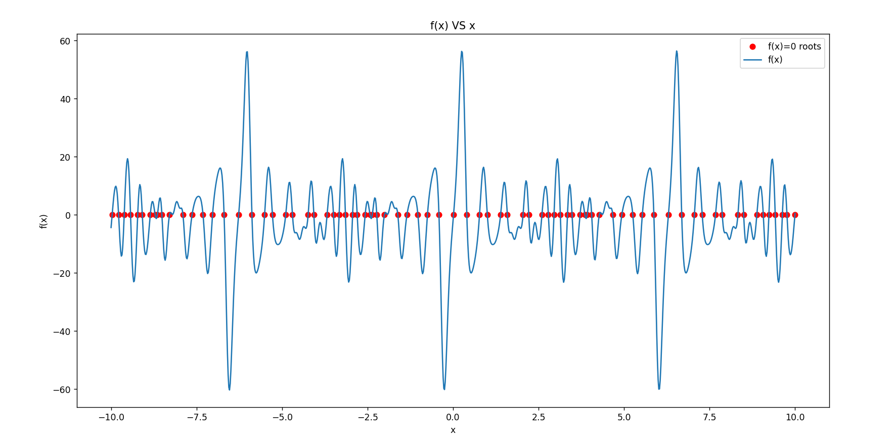
结果:
SecantMethod2Ps time:0.102962 s
展开
root_1 = -9.9674243605 , 误差 = -9.84635e-12
root_2 = -9.7797174668 , 误差 = 2.42473e-13
root_3 = -9.6149032646 , 误差 = -1.77636e-13
root_4 = -9.4302274624 , 误差 = -1.25011e-13
root_5 = -9.2207822340 , 误差 = -1.19016e-13
root_6 = -9.0871043561 , 误差 = 1.06581e-14
root_7 = -8.8530192104 , 误差 = -4.79616e-14
root_8 = -8.7125086779 , 误差 = 1.66800e-12
root_9 = -8.6442340327 , 误差 = -4.66294e-13
root_10 = -8.5133652799 , 误差 = -2.06057e-13
root_11 = -8.2899925123 , 误差 = 1.32339e-13
root_12 = -7.8981572477 , 误差 = 3.19744e-14
root_13 = -7.6307012374 , 误差 = 1.27010e-13
root_14 = -7.3115311582 , 误差 = 3.01981e-14
root_15 = -7.0320102646 , 误差 = 9.76117e-11
root_16 = -6.6955392638 , 误差 = -1.15463e-13
root_17 = -6.2691253474 , 误差 = -2.15383e-14
root_18 = -5.8813837698 , 误差 = 1.59872e-13
root_19 = -5.5099115066 , 误差 = -4.85390e-12
root_20 = -5.2816152128 , 误差 = -7.78790e-11
root_21 = -4.8929026655 , 误差 = -1.41718e-11
root_22 = -4.6958911893 , 误差 = -1.33227e-13
root_23 = -4.2373378929 , 误差 = -2.66454e-14
root_24 = -4.0708334564 , 误差 = -2.55929e-12
root_25 = -3.6842390533 , 误差 = -2.78444e-13
root_26 = -3.4965321596 , 误差 = 1.71951e-12
root_27 = -3.3317179574 , 误差 = 8.82672e-12
root_28 = -3.1470421552 , 误差 = -3.53051e-14
root_29 = -2.9375969268 , 误差 = 7.23333e-12
root_30 = -2.8039190490 , 误差 = -6.92779e-14
root_31 = -2.5698339033 , 误差 = 7.99361e-15
root_32 = -2.4293233707 , 误差 = 7.14540e-13
root_33 = -2.3610487255 , 误差 = -2.20712e-12
root_34 = -2.2301799727 , 误差 = -4.79616e-14
root_35 = -2.0068072051 , 误差 = 2.57572e-13
root_36 = -1.6149719405 , 误差 = 1.22569e-13
root_37 = -1.3475159302 , 误差 = -1.59872e-14
root_38 = -1.0283458510 , 误差 = -1.77636e-15
root_39 = -0.7488249575 , 误差 = 1.52420e-11
root_40 = -0.4123539566 , 误差 = 3.97655e-11
root_41 = 0.0140599598 , 误差 = -1.95399e-14
root_42 = 0.4018015374 , 误差 = 3.55271e-15
root_43 = 0.7732738006 , 误差 = -8.86402e-13
root_44 = 1.0015700944 , 误差 = -1.06581e-14
root_45 = 1.3902826416 , 误差 = -4.44089e-14
root_46 = 1.5872941179 , 误差 = -1.39124e-11
root_47 = 2.0458474143 , 误差 = -1.59872e-14
root_48 = 2.2123518508 , 误差 = 1.46549e-14
root_49 = 2.5989462538 , 误差 = -1.77423e-11
root_50 = 2.7866531475 , 误差 = 1.83187e-11
root_51 = 2.9514673498 , 误差 = -4.97380e-14
root_52 = 3.1361431519 , 误差 = 7.53486e-12
root_53 = 3.3455883803 , 误差 = 7.95701e-11
root_54 = 3.4792662582 , 误差 = -1.42109e-14
root_55 = 3.7133514039 , 误差 = -2.66454e-15
root_56 = 3.8538619365 , 误差 = -8.10463e-14
root_57 = 3.9221365817 , 误差 = -2.15294e-12
root_58 = 4.0530053345 , 误差 = 1.63514e-12
root_59 = 4.2763781021 , 误差 = 8.88178e-16
root_60 = 4.6682133667 , 误差 = 4.58478e-12
root_61 = 4.9356693770 , 误差 = 3.82272e-12
root_62 = 5.2548394562 , 误差 = -1.77636e-15
root_63 = 5.5343603497 , 误差 = -5.32907e-15
root_64 = 5.8708313505 , 误差 = 6.39488e-14
root_65 = 6.2972452669 , 误差 = 3.10862e-14
root_66 = 6.6849868445 , 误差 = -7.10543e-15
root_67 = 7.0564591078 , 误差 = 9.23706e-14
root_68 = 7.2847554016 , 误差 = 9.23706e-14
root_69 = 7.6734679488 , 误差 = -1.04192e-11
root_70 = 7.8704794251 , 误差 = 2.66454e-15
root_71 = 8.3290327215 , 误差 = -6.03961e-14
root_72 = 8.4955371580 , 误差 = -3.67466e-11
root_73 = 8.8821315610 , 误差 = -4.97105e-11
root_74 = 9.0698384547 , 误差 = 3.88916e-11
root_75 = 9.2346526569 , 误差 = 1.24345e-13
root_76 = 9.4193284591 , 误差 = -5.30687e-13
root_77 = 9.6287736875 , 误差 = 1.22569e-13
root_78 = 9.7624515654 , 误差 = 2.06057e-13
root_79 = 9.9965367111 , 误差 = 3.23874e-12
总结
计算耗时: 二分法>牛顿下山法>割线法
第三题
# 数值实验第三题
from formu_lib import *
import numpy as np
from matplotlib import pyplot as plt
def fa(x:float)->float:
return x**5-3*x-10
def dfa(x:float)->float:
return 5*x**4-3
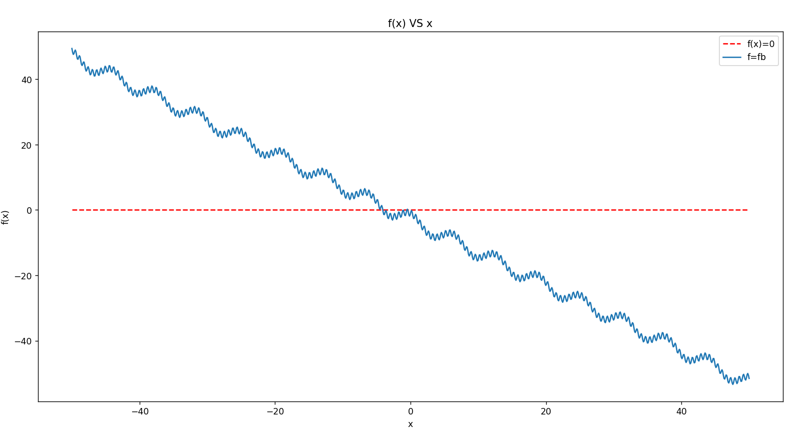
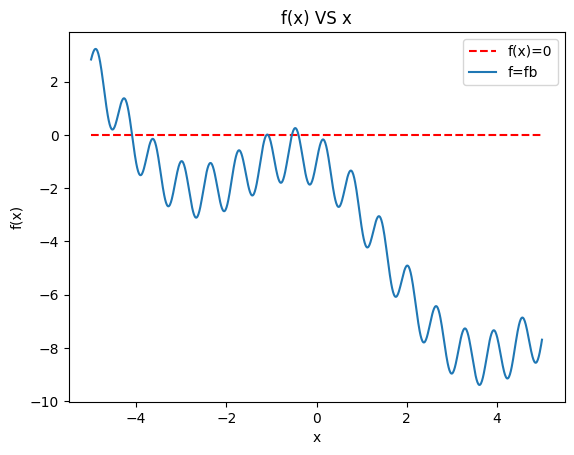
def fb(x:float)->float:
return np.sin(10*x)+2*np.cos(x)-x-3
def dfb(x:float)->float:
return 10*np.cos(10*x)-2*np.sin(x)-1
def fc(x:float)->float:
return x+np.arctan(x)-3
def dfc(x:float)->float:
return 1+1/(x**2+1)
def fd(x:float)->float:
return (x+2)*np.log(x*x+x+1)+1
def dfd(x:float)->float:
return np.log(x*x+x+1)+((2*x+1)*(x+2))/(x*x+x+1)
# initialize
a,b=-5,5
n=1000
tol=1e-10
plt.plot([a,b],[0,0],'r--',label='f(x)=0')
# 要计算的函数
f=fd
df=dfd
# 绘制原函数
x=np.linspace(a,b,n)
plt.plot(x,[f(i) for i in x],label=f'f={f.__name__}')
plt.xlabel('x')
plt.ylabel('f(x)')
plt.legend()
plt.title('f(x) VS x')
plt.show()
from time import time
st1=time()
rootEF=ComFormulaSolveNonlinearEquation(f,a,b,n,tol,'EF')
et1=time()
print(f"EF time:{(et1-st1):.6e} s ")
for ind,i in enumerate(rootEF):
print(f"root-{ind} : {i:.6e}")
st2=time()
rootND=ComFormulaSolveNonlinearEquation(f,a,b,n,tol,'ND',df)
et2=time()
print(f"ND time:{(et2-st2):.6e} s ")
for ind,i in enumerate(rootND):
print(f"root-{ind} : {i:.6e}")
st3=time()
rootGX=ComFormulaSolveNonlinearEquation(f,a,b,n,tol,'GX')
et3=time()
print(f"GX time:{(et3-st3):.6e} s ")
for ind,i in enumerate(rootGX):
print(f"root-{ind} : {i:.6e}")
st4=time()
rootNDXS=ComFormulaSolveNonlinearEquation(f,a,b,n,tol,'NDXS',df)
et4=time()
print(f"NDXS time:{(et4-st4):.6e} s ")
for ind,i in enumerate(rootNDXS):
print(f"root-{ind} : {i:.6e}")
(a)
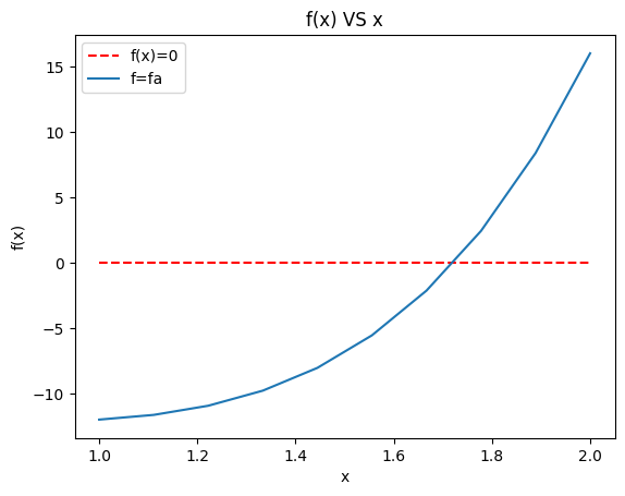
输出:
EF time:1.034021e-03 s , root:1.722600e+00
ND time:3.840923e-04 s , root:1.722600e+00
GX time:0.000000e+00 s , root:1.722600e+00
NDXS time:0.000000e+00 s , root:1.722600e+00
(b)
原函数:
输出:
EF time:1.297569e-02 s
root-0 : -4.091325e+00
root-1 : -1.106281e+00
root-2 : -1.077267e+00
root-3 : -5.443070e-01
root-4 : -4.001593e-01
ND time:9.279728e-03 s
root-0 : -4.091325e+00
root-1 : -1.106281e+00
root-2 : -1.077267e+00
root-3 : -5.443070e-01
root-4 : -4.001593e-01
GX time:7.452250e-03 s
root-0 : -4.091325e+00
root-1 : -1.106281e+00
root-2 : -1.077267e+00
root-3 : -5.443070e-01
root-4 : -4.001593e-01
NDXS time:6.772041e-03 s
root-0 : -4.091325e+00
root-1 : -1.106281e+00
root-2 : -1.077267e+00
root-3 : -5.443070e-01
root-4 : -4.001593e-01
(c)
原函数:
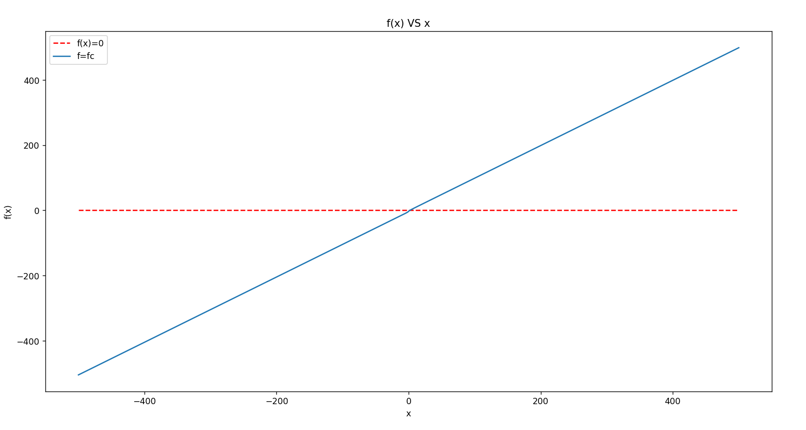
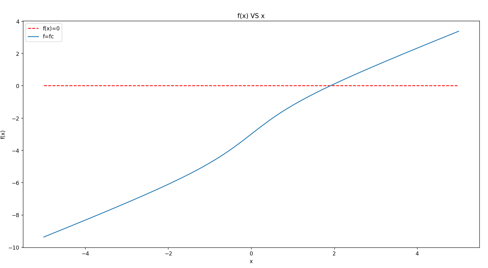
输出:
EF time:8.013487e-03 s
root-0 : 1.911252e+00
ND time:5.990267e-03 s
root-0 : 1.911252e+00
GX time:7.455111e-03 s
root-0 : 1.911252e+00
NDXS time:6.035566e-03 s
root-0 : 1.911252e+00
(d)
原函数:
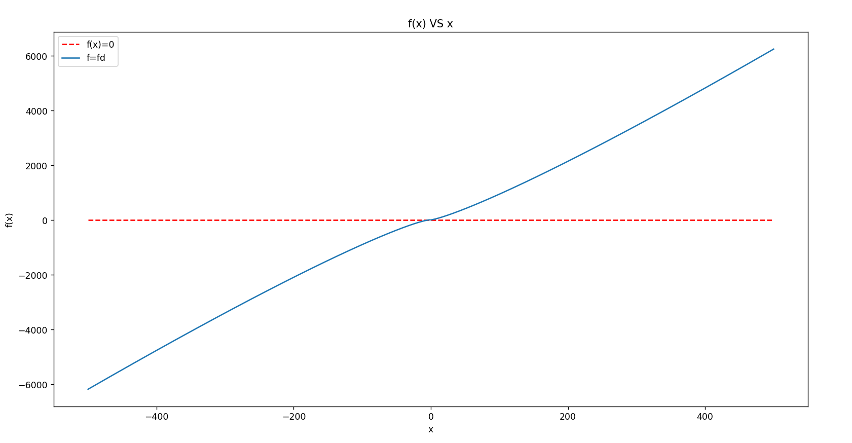
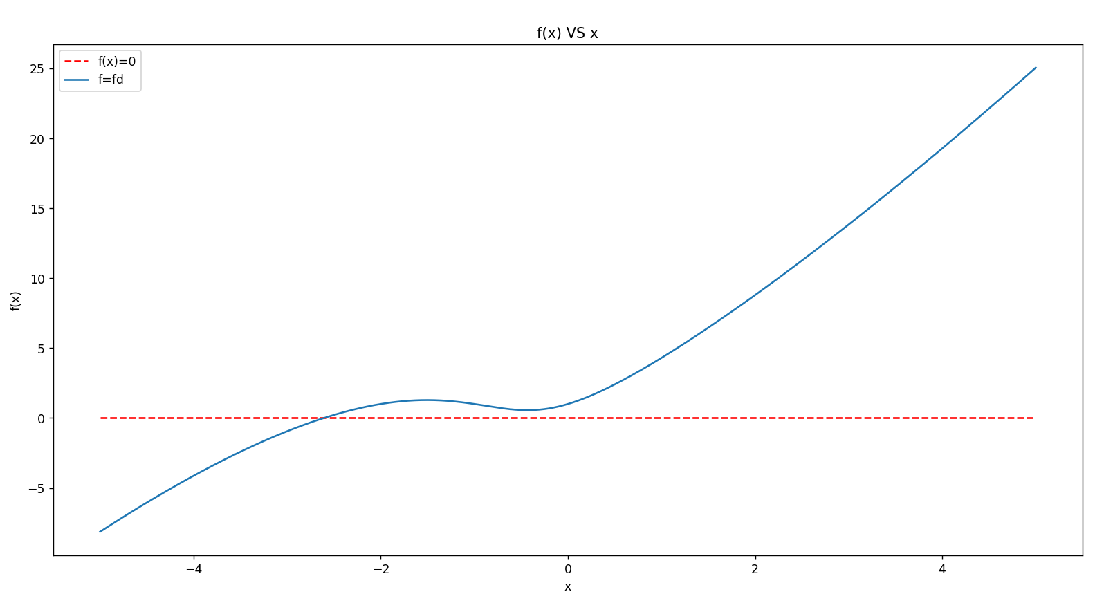
输出:
EF time:6.999493e-03 s
root-0 : -2.607232e+00
ND time:7.000446e-03 s
root-0 : -2.607232e+00
GX time:5.002499e-03 s
root-0 : -2.607232e+00
NDXS time:7.050514e-03 s
root-0 : -2.607232e+00
本文来自博客园,作者:FE-有限元鹰,转载请注明原文链接:https://www.cnblogs.com/aksoam/p/18355743

 浙公网安备 33010602011771号