
莫烦pytorch学习记录
感谢莫烦大神Pytorch B站视频:https://www.bilibili.com/video/av15997678?p=11
一个博主的笔记:https://blog.csdn.net/Will_Ye/article/details/104516423
一、PyTorch是什么?
它是一个基于Python的科学计算包,其主要是为了解决两类场景:
1、一种是可以替代Numpy进行科学计算,同时还可以使用张量在GPU上进行加速运算。
2、一个深度学习的研究平台,提供最大的灵活性和速度。
二、Numpy与Torch之间的转换

import torch
import numpy as np
from torch.autograd import Variable # torch 中 Variable 模块

### Torch 自称为神经网络界的 Numpy,
# 因为他能将 torch 产生的 tensor 放在 GPU 中加速运算
np_data = np.arange(6).reshape((2,3))
torch_data = torch.from_numpy(np_data) #torch形式
tensor2array = torch_data.numpy() # numpy形式
#  torch 做的和 numpy 能很好的兼容.
#  比如这样就能自由地转换 numpy array 和 torch tensor 了
print(
    '\nnumpy array:', np_data,  # [[0 1 2], [3 4 5]]
    '\ntorch tensor:', torch_data,  # 0  1  2 \n 3  4  5    [torch.LongTensor of size 2x3]
    '\ntensor to array:', tensor2array,  # [[0 1 2], [3 4 5]]
)
numpy array: [[0 1 2]
              [3 4 5]]
torch tensor: tensor([[0, 1, 2],
                      [3, 4, 5]], dtype=torch.int32)
tensor to array: [[0 1 2]
                  [3 4 5]]
三、Torch中的数学运算与numpy的对比
API手册
常用计算: 注意!!!!所有在pytorch里的计算,都要先转换为tensor的形式,不然就报错,切记!!!
#abs绝对值运算
data = [-1, -2, 1, 2]
tensor = torch.FloatTensor(data) # 转换成32位浮点tensor
print(
    '\nabs',
    '\nnumpy: ', np.abs(data),  # [1 2 1 2]
    '\ntorch: ', torch.abs(tensor)  # [1 2 1 2]
)

#sin 三角函数 sin
print(
    '\nsin',
    '\nnumpy: ', np.sin(data),  # [-0.84147098 -0.90929743  0.84147098  0.90929743]
    '\ntorch: ', torch.sin(tensor)  # [-0.8415 -0.9093  0.8415  0.9093]
)

#mean 均值
print(
    '\nmean',
    '\nnumpy: ', np.mean(data),         # 0.0
    '\ntorch: ', torch.mean(tensor)     # 0.0
)
矩阵计算:注意,有些numpy的封装的函数跟pytorch的不一样,这一点一定要区分清楚,也是很容易出问题的一个地方。
# matrix multiplication 矩阵点乘
data = [[1,2], [3,4]]
tensor = torch.FloatTensor(data)  # 转换成32位浮点 tensor
# correct method
print(
    '\nmatrix multiplication (matmul)',
    '\nnumpy: ', np.matmul(data, data),     # [[7, 10], [15, 22]]
    '\ntorch: ', torch.mm(tensor, tensor)   # [[7, 10], [15, 22]]
)

# !!!!  下面是错误的方法 !!!!
data = np.array(data)
print(
    '\nmatrix multiplication (dot)',
    '\nnumpy: ', data.dot(data),        # [[7, 10], [15, 22]] 在numpy 中可行
    # 关于 tensor.dot() 有了新的改变, 它只能针对于一维的数组. 所以上面的有所改变.
    # '\ntorch: ', tensor.dot(tensor)     # torch 会转换成 [1,2,3,4].dot([1,2,3,4) = 30.0
    # 变为
    # '\ntorch: ', torch.dot(tensor.dot(tensor))#
)
四、Variable
tensor = torch.FloatTensor([[1,2],[3,4]])
# 里面的值会不停的变化. 就像一个裝鸡蛋的篮子, 鸡蛋数会不停变动.
# 那谁是里面的鸡蛋呢, 自然就是 Torch 的 Tensor 咯.
# 如果用一个 Variable 进行计算, 那返回的也是一个同类型的 Variable.
# 把鸡蛋放到篮子里,
variable = Variable(tensor, requires_grad=True)#requires_grad是参不参与误差反向传播, 要不要计算梯度

print('\n',tensor)
"""
 1  2
 3  4
[torch.FloatTensor of size 2x2]
"""

print(variable)
"""
Variable containing:
 1  2
 3  4
[torch.FloatTensor of size 2x2]
"""
variable的计算
模仿一个计算梯度的情况
比较tensor的计算和variable的计算,在正向传播它们是看不出有什么不同的,而且variable和tensor有个很大的区别,variable是存储变量的,是会改变的,而tensor是不会改变的,是我们输入时就设定好的参数,variable会在反向传播后修正自己的数值。 这是我觉得他们最大的不同。
t_out = torch.mean(tensor*tensor)       # x^2
v_out = torch.mean(variable*variable)   # x^2
print('\n',t_out)
print('\n',v_out)    # 7.5
假设mean的均值做为结果的误差,对误差反向传播得到各项梯度。利用这个例子去看,在反向传播中它们之间的不同。
v_out = torch.mean(variable*variable)就是给各个variable搭建一个运算的步骤,搭建的网络也是其中一种运算的步骤。
v_out.backward()    # 模拟 v_out 的误差反向传递,在背景计算图中加速运算
# 下面两步看不懂没关系, 只要知道 Variable 是计算图的一部分, 可以用来传递误差就好.
# v_out = 1/4 * sum(variable*variable) 这是计算图中的 v_out 计算步骤
# 针对于 v_out 的梯度就是, d(v_out)/d(variable) = 1/4*2*variable = variable/2
print('\n',variable.grad)    # 初始 Variable 的梯度
'''
 0.5000  1.0000
 1.5000  2.0000
'''
可以看到,在backward中已经计算好梯度了,利用*.grad将背景中计算好的variable的各项梯度print出来。
这样如果是个网络的运算步骤也可以在backward中将各个梯度计算好。
获取Variable里面的数据
直接print(variable)只会输出 Variable形式的数据, 在很多时候是用不了的(比如想要用 plt 画图), 需要转换成tensor形式.
## 获取 Variable 里面的数据
print(variable)     #  Variable 形式
"""
Variable containing:
 1  2
 3  4
[torch.FloatTensor of size 2x2]
"""
print(variable.data)    # tensor 形式
"""
 1  2
 3  4
[torch.FloatTensor of size 2x2]
"""
print(variable.data.numpy())    # numpy 形式
"""
[[ 1.  2.]
 [ 3.  4.]]
"""
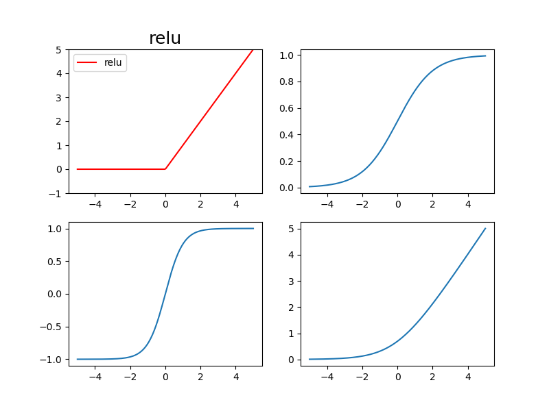
五、常用几种激励函数及图像
常用几种激励函数:relu, sigmoid, tanh, softplus
# 做一些假数据来观看图像
x = torch.linspace(-5, 5, 200)  # x data (tensor), shape=(100, 1)
x = Variable(x)
# Torch 中的激励函数有很多, 不过我们平时要用到的就这几个.
# relu, sigmoid, tanh, softplus. 那我们就看看他们各自长什么样啦.
x_np = x.data.numpy()   # 换成 numpy array, 出图时用
莫烦大神那时的版本用的是torch.nn.relu,但后来版本改了,直接用torch.relu就可以,其他激励函数也一样。
# 几种常用的 激励函数
y_relu = F.relu(x).data.numpy()
y_sigmoid = torch.sigmoid(x).data.numpy()
y_tanh = torch.tanh(x).data.numpy()
y_softplus = F.softplus(x).data.numpy()
# y_softmax = F.softmax(x)  softmax 比较特殊, 不能直接显示, 不过他是关于概率的, 用于分类
#用pit画 plt.figure(1,figsize=(8,6)) plt.subplot(221) plt.plot(x_np,y_relu, c='red', label='relu') plt.ylim(-1,5) plt.legend(loc='best') plt.subplot(222) plt.plot(x_np,y_sigmoid, c='red',label='sigmoid') plt.ylim(-0.2,1.2) plt.legend(loc='best') plt.subplot(223) plt.plot(x_np,y_tanh, c='red',label='tanh') plt.ylim(-1.2,1.2) plt.legend(loc='best') plt.subplot(224) plt.plot(x_np,y_softplus, c='red',label='softplus') plt.ylim(-0.2,6) plt.legend(loc='best')#用ax画 fig, ax = plt.subplots(2,2,figsize=(8,6)) ax[0,0].plot(x_np,y_relu,c='red', label='relu') ax[0,0].set_title('relu',fontsize=18) ax[0,0].set_ylim(-1,5) ax[0,0].legend() ax[0,1].plot(x_np,y_sigmoid) ax[1,0].plot(x_np,y_tanh) ax[1,1].plot(x_np,y_softplus) plt.show()
六、线性拟合回归
import torch
import matplotlib.pyplot as plt
import torch.nn.functional as F
#######捏造数据#######
x = torch.unsqueeze(torch.linspace(-1,1,500),dim=1)#x的数据,shape=(500,1)
y = x.pow(2) + 0.2*torch.rand(x.size())
# 画图看看捏的数据咋样
fig,ax = plt.subplots(2,1)
ax[0].scatter(x.data.numpy(),y.data.numpy())
ax[0].set_title("Pinched data",fontsize=18)
搭建网络
# 建立一个神经网络我们可以直接运用 torch 中的体系. 先定义所有的层属性(__init__()),
# 然后再一层层搭建(forward(x))层于层的关系链接. 建立关系的时候, 我们会用到激励函数.
class Net(torch.nn.Module): #继承torch中的Module
    def __init__(self,n_feature,n_hidden,n_output):
        super(Net, self).__init__() #继承__init__功能
        # 定义每层用什么样的形式
        self.hidden = torch.nn.Linear(n_feature,n_hidden) # 隐藏层线性输出
        self.predict = torch.nn.Linear(n_hidden,n_output)  # 输出层线性输出

    def forward(self,x): # 这同时也是Module中的forward功能
        # 正向传播输入值,神经网络分析出输出值
        x = F.relu(self.hidden(x))  # 激励函数(隐藏层的线性值)
        x = self.predict(x)         # 输出值
        return x

net = Net(n_feature=1, n_hidden=10, n_output=1)
print(net)
"""
Net (
  (hidden): Linear (1 -> 10)
  (predict): Linear (10 -> 1)
)
"""
开始训练
#optimizer训练工具
optimizer = torch.optim.SGD(net.parameters(), lr=0.2) # 传入net的所有参数,学习率
loss_func = torch.nn.MSELoss() # 预测值和真实值的误差计算公式(均方差)

plt.ion()
for t in range(10000):
    prediction = net(x) # 喂给net训练数据x,输出预测值
    loss = loss_func(prediction, y) # 计算两者的误差,#要预测值在前,label在后

    optimizer.zero_grad() # 清空上一步的残余更新参数值,#net.parameters()所有参数梯度变为0
    loss.backward()       # 误差反向传播,计算参数更新
    optimizer.step()      # 将参数更新施加到net的parameters上,#optimizr优化parameters
可视化训练过程
    if t % 5 == 0:
        # plot and show learning process
        ax[1].cla()
        ax[1].scatter(x.data.numpy(), y.data.numpy())
        ax[1].plot(x.data.numpy(), prediction.data.numpy(), 'r-', lw=5)
        ax[1].text(0.5, 0, 'Loss=%.4f' % loss.data.numpy(), fontdict={'size': 20, 'color': 'red'})
        plt.pause(0.01)
#如果在脚本中使用ion()命令开启了交互模式,没有使用ioff()关闭的话,
# 则图像会一闪而过,并不会常留。要想防止这种情况,需要在plt.show()之前加上ioff()命令。
plt.ioff()
plt.show()
七、区分类型 (分类)
捏个数据
import torch
import matplotlib.pyplot as plt

# 假数据
n_data = torch.ones(100, 2)         # 数据的基本形态
x0 = torch.normal(2*n_data, 1)      # 类型0 x data (tensor), shape=(100, 2)
y0 = torch.zeros(100)               # 类型0 y data (tensor), shape=(100, )
x1 = torch.normal(-2*n_data, 1)     # 类型1 x data (tensor), shape=(100, 1)
y1 = torch.ones(100)                # 类型1 y data (tensor), shape=(100, )

# 注意 x, y 数据的数据形式是一定要像下面一样 (torch.cat 是在合并数据)
x = torch.cat((x0, x1), 0).type(torch.FloatTensor)  # FloatTensor = 32-bit floating
y = torch.cat((y0, y1), ).type(torch.LongTensor)    # LongTensor = 64-bit integer


# 画图 会出错:会报错,因为画图x和y的数量不相同,x矩阵的形状是(200,2)的,而y矩阵的形状是(200),
# 所以需要把x分成两部分来画图才可以的。
# plt.scatter(x.data.numpy(), y.data.numpy())
# plt.show()
# 画图
plt.scatter(x.data.numpy()[:, 0], x.data.numpy()[:, 1], c=y.data.numpy(), s=100, lw=0, cmap='RdYlGn')
plt.show()
搭个网络
class Net(torch.nn.Module):
    def __init__(self,n_feature,n_hidden,n_outpot):
        super(Net,self).__init__()  #继承__init__的功能
        self.hidden = torch.nn.Linear(n_feature,n_hidden)
        self.out = torch.nn.Linear(n_hidden,n_outpot)

    def forward(self,x):
        x = torch.relu(self.hidden(x))
        x = self.out(x)
        return x

net = Net(n_feature=2,n_hidden=10,n_outpot=2)

print(net)
训练网络
optimizer = torch.optim.SGD(net.parameters(), lr=0.02)  # 传入 net 的所有参数, 学习率
# 算误差的时候, 注意真实值!不是! one-hot 形式的, 而是1D Tensor, (batch,)
# 但是预测值是2D tensor (batch, n_classes)
loss_func = torch.nn.CrossEntropyLoss()

for t in range(100):
    out = net(x)     # 喂给 net 训练数据 x, 输出分析值

    loss = loss_func(out, y)     # 计算两者的误差

    optimizer.zero_grad()   # 清空上一步的残余更新参数值
    loss.backward()         # 误差反向传播, 计算参数更新值
    optimizer.step()        # 将参数更新值施加到 net 的 parameters 上
可视化
plt.ion()
for t in range(100):
    out = net(x)     # 喂给 net 训练数据 x, 输出分析值

    loss = loss_func(out, y)     # 计算两者的误差

    optimizer.zero_grad()   # 清空上一步的残余更新参数值
    loss.backward()         # 误差反向传播, 计算参数更新值
    optimizer.step()        # 将参数更新值施加到 net 的 parameters 上
    # 接着上面来
    if t % 2 == 0:
        plt.cla()
        # 过了一道 softmax 的激励函数后的最大概率才是预测值
        prediction = torch.max(F.softmax(out), 1)[1]
        #prediction=torch.max(F.softmax(out), 1) 中的1,表示【0,0,1】预测结果中,结果为1的结果的位置。
        pred_y = prediction.data.numpy().squeeze()#利用squeeze()函数将表示向量的数组转换为秩为1的数组,这样利用matplotlib库函数画图时,就可以正常的显示结果了
        target_y = y.data.numpy()
        plt.scatter(x.data.numpy()[:, 0], x.data.numpy()[:, 1], c=pred_y, s=100, lw=0, cmap='RdYlGn')
        accuracy = sum(pred_y == target_y) / 200.  # 预测中有多少和真实值一样
        plt.text(1.5, -4, 'Accuracy=%.2f' % accuracy, fontdict={'size': 20, 'color': 'red'})
        plt.pause(0.1)

plt.ioff()
plt.show()
八、快速搭建法
Torch 中提供了很多方便的途径, 同样是神经网络, 能快则快, 我们看看如何用更简单的方式搭建同样的回归神经网络.
上一节用的方法更加底层,其实有更加快速的方法,对比一下就很清楚了:
Method 1
我们用 class 继承了一个 torch 中的神经网络结构, 然后对其进行了修改
class Net(torch.nn.Module): #我们用 class 继承了一个 torch 中的神经网络结构, 然后对其进行了修改
    def __init__(self,n_feature,n_hidden,n_outpot):
        super(Net,self).__init__()  #继承__init__的功能,
        self.hidden = torch.nn.Linear(n_feature,n_hidden)
        self.out = torch.nn.Linear(n_hidden,n_outpot)

    def forward(self,x):
        x = torch.relu(self.hidden(x))
        x = self.out(x)
        return x

net1 = Net(n_feature=2,n_hidden=10,n_outpot=2)
Method 2
用nn库里一个函数就能快速搭建了,注意ReLU也算做一层加入到网络序列中
net2 = torch.nn.Sequential(
    torch.nn.Linear(2,10),
    torch.nn.ReLU(),
    torch.nn.Linear(10,2)
)
print(net1)
print(net2)
结果是类似的:就是net2中将ReLU也做为一个神经层
print(net1)
"""
Net(
  (hidden): Linear(in_features=2, out_features=10, bias=True)
  (out): Linear(in_features=10, out_features=2, bias=True)
)
"""
print(net2)
"""
Sequential(
  (0): Linear(in_features=2, out_features=10, bias=True)
  (1): ReLU()
  (2): Linear(in_features=10, out_features=2, bias=True)
)
"""
九、保存与提取网络
保存
#######捏造数据#######
torch.manual_seed(1)    # reproducible 使得每次随机初始化的随机数是一致的
x = torch.unsqueeze(torch.linspace(-1,1,500),dim=1)#x的数据,shape=(500,1)
y = x.pow(2) + 0.2*torch.rand(x.size())

def save():
    # 搭建网络
    net1 = torch.nn.Sequential(
        torch.nn.Linear(1, 10),
        torch.nn.ReLU(),
        torch.nn.Linear(10, 1),
    )
    optimizer = torch.optim.SGD(net1.parameters(), lr=0.5)
    loss_func = torch.nn.MSELoss()
    # 训练
    for t in range(100):
        prediction = net1(x)
        loss = loss_func(prediction, y)
        optimizer.zero_grad()
        loss.backward()
        optimizer.step()

    torch.save(net1, 'net.pkl')  # 保存整个网络
    torch.save(net1.state_dict(), 'net_params.pkl')  # 只保存网络中的参数 (速度快, 占内存少)
提取网络
# 这种方式将会提取整个神经网络, 网络大的时候可能会比较慢.
def restore_net():
    # restore entire net1 to net2
    net2 = torch.load('net.pkl')
    prediction = net2(x)
只提取网络参数
# 这种方式将会提取所有的参数, 然后再放到你的新建网络中.
def restore_params():
    # 新建 net3
    net3 = torch.nn.Sequential(
        torch.nn.Linear(1, 10),
        torch.nn.ReLU(),
        torch.nn.Linear(10, 1)
    )

    # 将保存的参数复制到 net3
    net3.load_state_dict(torch.load('net_params.pkl'))
    prediction = net3(x)
完整代码并查看三个网络模型的结果
import torch
import matplotlib.pyplot as plt
import torch.nn.functional as F
from matplotlib import animation
#######捏造数据#######
torch.manual_seed(1)    # reproducible 使得每次随机初始化的随机数是一致的
x = torch.unsqueeze(torch.linspace(-1,1,100),dim=1)#x的数据,shape=(500,1)
y = x.pow(2) + 0.2*torch.rand(x.size())


def save():
    # 搭建网络
    net1 = torch.nn.Sequential(
        torch.nn.Linear(1, 100),
        torch.nn.ReLU(),
        torch.nn.Linear(100, 1),
    )
    optimizer = torch.optim.SGD(net1.parameters(), lr=0.3)
    loss_func = torch.nn.MSELoss()
    # 训练
    for t in range(1000):
        prediction = net1(x)
        loss = loss_func(prediction, y)
        optimizer.zero_grad()
        loss.backward()
        optimizer.step()

    torch.save(net1, 'net.pkl')  # 保存整个网络
    torch.save(net1.state_dict(), 'net_params.pkl')  # 只保存网络中的参数 (速度快, 占内存少)

    # plot result
    plt.figure(1, figsize=(10,3))
    plt.subplot(131)
    plt.title('Net1')
    plt.scatter(x.data.numpy(), y.data.numpy())
    plt.plot(x.data.numpy(), prediction.data.numpy(), 'r-', lw=5)


# 这种方式将会提取整个神经网络, 网络大的时候可能会比较慢.
def restore_net():
    # restore entire net1 to net2
    net2 = torch.load('net.pkl')
    prediction = net2(x)

    # plot result
    plt.figure(1, figsize=(10,3))
    plt.subplot(132)
    plt.title('Net2')
    plt.scatter(x.data.numpy(), y.data.numpy())
    plt.plot(x.data.numpy(), prediction.data.numpy(), 'r-', lw=5)

# 这种方式将会提取所有的参数, 然后再放到你的新建网络中.
def restore_params():
    # 新建 net3
    net3 = torch.nn.Sequential(
        torch.nn.Linear(1, 100),
        torch.nn.ReLU(),
        torch.nn.Linear(100, 1)
    )

    # 将保存的参数复制到 net3
    net3.load_state_dict(torch.load('net_params.pkl'))
    prediction = net3(x)
    # plot result
    plt.figure(1, figsize=(10,3))
    plt.subplot(133)
    plt.title('Net3')
    plt.scatter(x.data.numpy(), y.data.numpy())
    plt.plot(x.data.numpy(), prediction.data.numpy(), 'r-', lw=5)


# 保存 net1 (1. 整个网络, 2. 只有参数)
save()

# 提取整个网络
restore_net()

# 提取网络参数, 复制到新网络
restore_params()

plt.show()

十、批训练
进行批量训练需要用到一个很好用的工具DataLoader 。
注意,莫烦大神用的版本跟现在新版还是有些出入的,用Data.TensorDataset这个函数,不要指定data_tensor和target_tensor会报错的,因为新版的库改了,直接输入x和y就行了。
数据分批
import torch
import torch.utils.data as tud
torch.manual_seed(1)

BATCH_SIZE = 20  #批训练的数据个数,每批20个
#######捏造数据#######
x = torch.unsqueeze(torch.linspace(-1,1,100),dim=1)#x的数据,shape=(100,1)
y = x.pow(2) + 0.2*torch.rand(x.size())

# 先转换成 torch 能识别的 Dataset
# torch_dataset = DL.TensorDataset(data_tensor=x, target_tensor=y)
# 新版的库改了,直接输入x和y就行了。
torch_dataset = tud.TensorDataset(x,y)

# 把dataset放入DataLoader
loader = tud.DataLoader(
    dataset=torch_dataset, # 转换好的torch能识别的dataset导入DataLoader
    batch_size=BATCH_SIZE, # 每批的大小是多大
    shuffle=True,          # 要不要打乱数据顺序(一般打乱比较好)
    num_workers=2          # 多线程来读取数据

)
分批训练
epoch表示整体数据训练次数,step则是每一批数据里面有几组数据
def show_batch():
    for epoch in range(3):     # 训练所有!整套!数据3次
        for step,(batch_x, batch_y) in enumerate(loader): #每一步loader释放一批数据来学习
            # 训练的地方

            # 打出来一些数据
            print('Epoch:',epoch,'|Step:',step,'|batch x:',batch_x.numpy(),'|batch y:',batch_y.numpy())

if __name__ == '__main__':
    show_batch()
"""
Epoch: 0 |Step: 0 |batch x: [ 5.  7. 10.  3.  4.] |batch y: [6. 4. 1. 8. 7.]
Epoch: 0 |Step: 1 |batch x: [2. 1. 8. 9. 6.] |batch y: [ 9. 10.  3.  2.  5.]
Epoch: 1 |Step: 0 |batch x: [ 4.  6.  7. 10.  8.] |batch y: [7. 5. 4. 1. 3.]
Epoch: 1 |Step: 1 |batch x: [5. 3. 2. 1. 9.] |batch y: [ 6.  8.  9. 10.  2.]
Epoch: 2 |Step: 0 |batch x: [ 4.  2.  5.  6. 10.] |batch y: [7. 9. 6. 5. 1.]
Epoch: 2 |Step: 1 |batch x: [3. 9. 1. 8. 7.] |batch y: [ 8.  2. 10.  3.  4.]
"""
可以看出, 每步都导出了5个数据进行学习. 然后每个 epoch 的导出数据都是先打乱了以后再导出。
改变一下 BATCH_SIZE = 8, 这样我们就知道, step=0 会导出8个数据, 但是, step=1 时数据库中的数据不够 8个, 这时怎么办呢:这时, 在 step=1 就只给你返回这个 epoch 中剩下的数据就好了.
Epoch: 0 |Step: 0 |batch x: [ 5.  7. 10.  3.  4.  2.  1.  8.] |batch y: [ 6.  4.  1.  8.  7.  9. 10.  3.]
Epoch: 0 |Step: 1 |batch x: [9. 6.] |batch y: [2. 5.]
Epoch: 1 |Step: 0 |batch x: [ 4.  6.  7. 10.  8.  5.  3.  2.] |batch y: [7. 5. 4. 1. 3. 6. 8. 9.]
Epoch: 1 |Step: 1 |batch x: [1. 9.] |batch y: [10.  2.]
Epoch: 2 |Step: 0 |batch x: [ 4.  2.  5.  6. 10.  3.  9.  1.] |batch y: [ 7.  9.  6.  5.  1.  8.  2. 10.]
Epoch: 2 |Step: 1 |batch x: [8. 7.] |batch y: [3. 4.]
十一、Optimizer 优化器
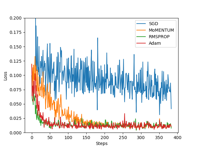
各种不同的优化器 在同一个网路上的对比
SGD 是最普通的优化器, 也可以说没有加速效果, 而 Momentum 是 SGD 的改良版, 它加入了动量原则. 后面的 RMSprop 又是 Momentum 的升级版. 而 Adam 又是 RMSprop 的升级版. 不过从这个结果中我们看到, Adam 的效果似乎比 RMSprop 要差一点. 所以说并不是越先进的优化器, 结果越佳.
1.捏一个数据
import torch
import torch.utils.data as tud
import matplotlib.pyplot as plt

torch.manual_seed(1)

LR = 0.01
BATCH_SIZE = 32
EPOCH = 12

######捏一个数据######
x = torch.unsqueeze(torch.linspace(-1,1,1000),dim=1)
y = x.pow(2) + 0.1*torch.normal(torch.zeros(*x.size()))

plt.scatter(x.numpy(),y.numpy())
plt.show()
torch_dataset = tud.TensorDataset(x,y)
loader = tud.DataLoader(
    dataset=torch_dataset,
    batch_size=BATCH_SIZE,
    shuffle=True,
    num_workers=2
)
2.建立同样的网络
# 搭建同样的网络Net
class Net(torch.nn.Module):
    def __init__(self):
        super(Net, self).__init__()
        self.hidden = torch.nn.Linear(1,20)
        self.predict = torch.nn.Linear(20,1)

    def forward(self,x):
        x = torch.ReLU(self.hidden(x))
        x = self.predict(x)
        return  x
# 为每个优化器创建一个net
net_SGD = Net()
net_Momentum = Net()
net_RMSprop = Net()
net_Adam = Net()
nets = [net_SGD,net_Momentum,net_RMSprop,net_Adam]
3.不同的optimizer
接下来在创建不同的优化器, 用来训练不同的网络. 并创建一个 loss_func 用来计算误差. 我们用几种常见的优化器, SGD, Momentum, RMSprop, Adam.
# different optimizers
opt_SGD         = torch.optim.SGD(net_SGD.parameters(), lr=LR)
opt_Momentum    = torch.optim.SGD(net_Momentum.parameters(), lr=LR, momentum=0.8)
opt_RMSprop     = torch.optim.RMSprop(net_RMSprop.parameters(), lr=LR, alpha=0.9)
opt_Adam        = torch.optim.Adam(net_Adam.parameters(), lr=LR, betas=(0.9, 0.99))
optimizers = [opt_SGD, opt_Momentum, opt_RMSprop, opt_Adam]

loss_func = torch.nn.MSELoss()
losses_his = [[], [], [], []]   # 记录 training 时不同神经网络的 loss
4.训练出图
    for epoch in range(EPOCH):
        print('Epoch',epoch)
        for step,(b_x,b_y) in enumerate(loader):
            # 对每个优化器, 优化属于他的神经网络
            for net, opt, l_his in zip(nets, optimizers, losses_his):
                output = net(b_x)  # 获得每个网络的输出
                loss = loss_func(output, b_y)  # compute loss for every net
                opt.zero_grad()  # clear gradients for next train
                loss.backward()  # backpropagation, compute gradients
                opt.step()  # apply gradients
                l_his.append(loss.data.numpy())  # loss recoder

    labels = ['SGD', 'MoMENTUM', 'RMSPROP', 'Adam']
    for i, l_his in enumerate(losses_his):
        plt.plot(l_his, label=labels[i])
    plt.legend(loc='best')
    plt.xlabel('Steps')
    plt.ylabel('Loss')
    plt.ylim((0, 0.2))
    plt.show()
完整代码
import torch
import torch.utils.data as tud
import matplotlib.pyplot as plt
import torch.nn.functional as F
torch.manual_seed(1)

LR = 0.01
BATCH_SIZE = 32
EPOCH = 12

######捏一个数据######
x = torch.unsqueeze(torch.linspace(-1,1,1000),dim=1)
y = x.pow(2) + 0.1*torch.normal(torch.zeros(*x.size()))

# plt.scatter(x.numpy(),y.numpy())
# plt.show()

torch_dataset = tud.TensorDataset(x,y)
loader = tud.DataLoader(
    dataset=torch_dataset,
    batch_size=BATCH_SIZE,
    shuffle=True,
    num_workers=2
)

# 搭建同样的网络Net
class Net(torch.nn.Module):
    def __init__(self):
        super(Net, self).__init__()
        self.hidden = torch.nn.Linear(1,20)
        self.predict = torch.nn.Linear(20,1)

    def forward(self,x):
        x = F.relu(self.hidden(x))
        x = self.predict(x)
        return  x

if __name__== '__main__':
    # 为每个优化器创建一个net
    net_SGD = Net()
    net_Momentum = Net()
    net_RMSprop = Net()
    net_Adam = Net()
    nets = [net_SGD,net_Momentum,net_RMSprop,net_Adam]

    # different optimizers
    opt_SGD         = torch.optim.SGD(net_SGD.parameters(), lr=LR)
    opt_Momentum    = torch.optim.SGD(net_Momentum.parameters(), lr=LR, momentum=0.8)
    opt_RMSprop     = torch.optim.RMSprop(net_RMSprop.parameters(), lr=LR, alpha=0.9)
    opt_Adam        = torch.optim.Adam(net_Adam.parameters(), lr=LR, betas=(0.9, 0.99))
    optimizers = [opt_SGD, opt_Momentum, opt_RMSprop, opt_Adam]

    loss_func = torch.nn.MSELoss()
    losses_his = [[], [], [], []]   # 记录 training 时不同神经网络的 loss

    for epoch in range(EPOCH):
        print('Epoch',epoch)
        for step,(b_x,b_y) in enumerate(loader):
            # 对每个优化器, 优化属于他的神经网络
            for net, opt, l_his in zip(nets, optimizers, losses_his):
                output = net(b_x)  # 获得每个网络的输出
                loss = loss_func(output, b_y)  # compute loss for every net
                opt.zero_grad()  # clear gradients for next train
                loss.backward()  # backpropagation, compute gradients
                opt.step()  # apply gradients
                l_his.append(loss.data.numpy())  # loss recoder

    labels = ['SGD', 'MoMENTUM', 'RMSPROP', 'Adam']
    for i, l_his in enumerate(losses_his):
        plt.plot(l_his, label=labels[i])
    plt.legend(loc='best')
    plt.xlabel('Steps')
    plt.ylabel('Loss')
    plt.ylim((0, 0.2))
    plt.show()
十二、CNN_classification
1、MINIST手写数据
import torch
import torch.nn as nn
import torch.utils.data as Data
import torchvision      # 数据库模块
import matplotlib.pyplot as plt

torch.manual_seed(1)    # reproducible

# Hyper Parameters
EPOCH = 1           # 训练整批数据多少次, 为了节约时间, 我们只训练一次
BATCH_SIZE = 50
LR = 0.001          # 学习率
DOWNLOAD_MNIST = True  # 如果你已经下载好了mnist数据就写上 False


# Mnist 手写数字
train_data = torchvision.datasets.MNIST(
    root='./mnist/',    # 保存或者提取位置
    train=True,  # this is training data
    transform=torchvision.transforms.ToTensor(),    # 转换 PIL.Image or numpy.ndarray 成
                                                    # torch.FloatTensor (C x H x W), 训练的时候 normalize 成 [0.0, 1.0] 区间
    download=DOWNLOAD_MNIST,          # 没下载就下载, 下载了就不用再下了
)

test_data = torchvision.datasets.MNIST(root='./mnist/', train=False)

# 批训练 50samples, 1 channel, 28x28 (50, 1, 28, 28)
train_loader = Data.DataLoader(dataset=train_data, batch_size=BATCH_SIZE, shuffle=True)

# 为了节约时间, 我们测试时只测试前2000个
test_x = torch.unsqueeze(test_data.test_data, dim=1).type(torch.FloatTensor)[:2000]/255.   # shape from (2000, 28, 28) to (2000, 1, 28, 28), value in range(0,1)
test_y = test_data.test_labels[:2000]
2、CNN模型
和以前一样, 我们用一个 class 来建立 CNN 模型. 这个 CNN 整体流程是
卷积(Conv2d) -> 激励函数(ReLU) -> 池化, 向下采样 (MaxPooling)
-> 再来一遍 -> 展平多维的卷积成的特征图 -> 接入全连接层 (Linear) -> 输出
# CNN模型搭建
class CNN(nn.Module):
    def __init__(self):
        super(CNN, self).__init__()
        self.conv1 = nn.Sequential(  # input shape (1,28,28)
            nn.Conv2d(
                in_channels=1,    # 输入高度
                out_channels=16,  # n_filters 输出高度
                kernel_size=5,    # 卷积核大小  filter size
                stride=1,         # 卷积核步进或者说步长,filter movement/step
                padding=2,        # 如果想要 con2d 出来的图片长宽没有变化, padding=(kernel_size-1)/2 当 stride=1

            ), ## output shape (16, 28, 28)
            nn.ReLU(),            # activation
            nn.MaxPool2d(kernel_size=2), #在2*2 空间里向下采样,output shape (16, 14, 14)
        )
        self.conv2 = nn.Sequential(   # input shape (16,14,14)
            nn.Conv2d(16,32,5,1,2),   # output shape(32,14,14)
            nn.ReLU(),
            nn.MaxPool2d(2),          # output size (32,7,7)
        )
        self.out = nn.Linear(32*7*7,10)  # 全连接层输出10个类
    def forword(self,x):
        x = self.conv1(x)
        x = self.conv2(x)
        x = x.view(x.size(0), -1) # 展平多维的卷积图成 (batch_size, 32 * 7 * 7)
        output = self.out(x)
        return output

cnn = CNN()
print(cnn)
CNN(
  (conv1): Sequential(
    (0): Conv2d(1, 16, kernel_size=(5, 5), stride=(1, 1), padding=(2, 2))
    (1): ReLU()
    (2): MaxPool2d(kernel_size=2, stride=2, padding=0, dilation=1, ceil_mode=False)
  )
  (conv2): Sequential(
    (0): Conv2d(16, 32, kernel_size=(5, 5), stride=(1, 1), padding=(2, 2))
    (1): ReLU()
    (2): MaxPool2d(kernel_size=2, stride=2, padding=0, dilation=1, ceil_mode=False)
  )
  (out): Linear(in_features=1568, out_features=10, bias=True)
)
3、训练,全部代码
下面我们开始训练, 将 x y 都用 Variable 包起来, 然后放入 cnn 中计算 output, 最后再计算误差.下面代码省略了计算精确度 accuracy 的部分
import os
import torch
import torch.nn as nn
import torch.utils.data as Data
import torchvision      # 数据库模块
import matplotlib.pyplot as plt
from matplotlib import cm

torch.manual_seed(1)    # reproducible

# Hyper Parameters
EPOCH = 1           # 训练整批数据多少次, 为了节约时间, 我们只训练一次
BATCH_SIZE = 50
LR = 0.001          # 学习率
DOWNLOAD_MNIST = False  # 如果你已经下载好了mnist数据就写上 False

if not(os.path.exists('./mnist/')) or not os.listdir('./mnist/'):
    # not mnist dir or mnist is empyt dir
    DOWNLOAD_MNIST = True


# Mnist 手写数字
train_data = torchvision.datasets.MNIST(
    root='./mnist/',    # 保存或者提取位置
    train=True,  # this is training data
    transform=torchvision.transforms.ToTensor(),    # 转换 PIL.Image or numpy.ndarray 成
                                                    # torch.FloatTensor (C x H x W), 训练的时候 normalize 成 [0.0, 1.0] 区间
    download=DOWNLOAD_MNIST,          # 没下载就下载, 下载了就不用再下了
)

test_data = torchvision.datasets.MNIST(root='./mnist/', train=False)

# plot one example
print(train_data.data.size())                 # (60000, 28, 28)
print(train_data.targets.size())               # (60000)
plt.imshow(train_data.data[0].numpy(), cmap='gray')
plt.title('%i' % train_data.targets[0])
plt.show()


# 批训练 50samples, 1 channel, 28x28 (50, 1, 28, 28)
train_loader = Data.DataLoader(dataset=train_data, batch_size=BATCH_SIZE, shuffle=True)

# 为了节约时间, 我们测试时只测试前2000个
test_x = torch.unsqueeze(test_data.data, dim=1).type(torch.FloatTensor)[:2000]/255.   # shape from (2000, 28, 28) to (2000, 1, 28, 28), value in range(0,1)
test_y = test_data.targets[:2000]

# CNN模型搭建
class CNN(nn.Module):
    def __init__(self):
        super(CNN, self).__init__()
        self.conv1 = nn.Sequential(  # input shape (1,28,28)
            nn.Conv2d(
                in_channels=1,    # 输入高度
                out_channels=16,  # n_filters 输出高度
                kernel_size=5,    # 卷积核大小  filter size
                stride=1,         # 卷积核步进或者说步长,filter movement/step
                padding=2,        # 如果想要 con2d 出来的图片长宽没有变化, padding=(kernel_size-1)/2 当 stride=1

            ), ## output shape (16, 28, 28)
            nn.ReLU(),            # activation
            nn.MaxPool2d(kernel_size=2), #在2*2 空间里向下采样,output shape (16, 14, 14)
        )
        self.conv2 = nn.Sequential(   # input shape (16,14,14)
            nn.Conv2d(16,32,5,1,2),   # output shape(32,14,14)
            nn.ReLU(),
            nn.MaxPool2d(2),          # output size (32,7,7)
        )
        self.out = nn.Linear(32*7*7,10)  # 全连接层输出10个类

    def forward(self,x):
        x = self.conv1(x)
        x = self.conv2(x)
        x = x.view(x.size(0), -1) # 展平多维的卷积图成 (batch_size, 32 * 7 * 7)
        output = self.out(x)
        return output, x


def train_save():
    cnn = CNN()
    print(cnn)

    optimizer = torch.optim.Adam(cnn.parameters(), lr=LR) # 优化整一个CNN的参数
    loss_func = nn.CrossEntropyLoss()

    try:
        from sklearn.manifold import TSNE;HAS_SK = True
    except:
        HAS_SK = False;
        print('Please install sklearn for layer visualization')

    def plot_with_labels(lowDWeights, labels):
        plt.cla()
        X, Y = lowDWeights[:, 0], lowDWeights[:, 1]
        for x, y, s in zip(X, Y, labels):
            c = cm.rainbow(int(255 * s / 9));
            plt.text(x, y, s, backgroundcolor=c, fontsize=9)
        plt.xlim(X.min(), X.max());
        plt.ylim(Y.min(), Y.max());
        plt.title('Visualize last layer');
        plt.show();
        plt.pause(0.01)

    plt.ion()

    # training and testing
    for epoch in range(EPOCH):
        for step, (b_x, b_y) in enumerate(train_loader):   # gives batch data, normalize x when iterate train_loader

            output = cnn(b_x)[0]            # cnn output
            loss = loss_func(output, b_y)   # cross entropy loss
            optimizer.zero_grad()           # clear gradients for this training step
            loss.backward()                 # backpropagation, compute gradients
            optimizer.step()                # apply gradients

            if step % 50 == 0:
                test_output, last_layer = cnn(test_x)
                pred_y = torch.max(test_output, 1)[1].data.numpy()
                accuracy = float((pred_y == test_y.data.numpy()).astype(int).sum()) / float(test_y.size(0))
                print('Epoch: ', epoch, '| train loss: %.4f' % loss.data.numpy(), '| test accuracy: %.2f' % accuracy)
                if HAS_SK:
                    # Visualization of trained flatten layer (T-SNE)
                    tsne = TSNE(perplexity=30, n_components=2, init='pca', n_iter=5000)
                    plot_only = 500
                    low_dim_embs = tsne.fit_transform(last_layer.data.numpy()[:plot_only, :])
                    labels = test_y.numpy()[:plot_only]
                    plot_with_labels(low_dim_embs, labels)
    plt.ioff()

    torch.save(cnn, './mnist_net/cnn_classification_net.pkl')  # 保存整个网络
    torch.save(cnn.state_dict(), './mnist_net/cnn_classification_net_params.pkl')  # 只保存网络中的参数 (速度快, 占内存少)

    """
    ...
    Epoch:  0 | train loss: 0.0306 | test accuracy: 0.97
    Epoch:  0 | train loss: 0.0147 | test accuracy: 0.98
    Epoch:  0 | train loss: 0.0427 | test accuracy: 0.98
    Epoch:  0 | train loss: 0.0078 | test accuracy: 0.98
    """

    # print 10 predictions from test data
    test_output, _ = cnn(test_x[:10])
    pred_y = torch.max(test_output, 1)[1].data.numpy()
    print(pred_y, 'prediction number')
    print(test_y[:10].numpy(), 'real number')
    """
    [7 2 1 0 4 1 4 9 5 9] prediction number
    [7 2 1 0 4 1 4 9 5 9] real number
    """


# 这种方式将会提取整个神经网络, 网络大的时候可能会比较慢.
def restore_net():
    # restore entire net1 to net2
    net2 = torch.load('./mnist_net/cnn_classification_net.pkl')
    test_output, _ = net2(test_x[:20])
    pred_y = torch.max(test_output, 1)[1].data.numpy()
    print(pred_y, 'prediction number')
    print(test_y[:20].numpy(), 'real number')

if __name__ == '__main__':
    train = True
    if train:
        train_save()
    else:
        restore_net()
十三、RNN_classification
1、MINIST手写数据
import os
import torch
import torch.nn as nn
import torch.utils.data as Data
import torchvision      # 数据库模块
import matplotlib.pyplot as plt
from matplotlib import cm
import torchvision.transforms as transforms
torch.manual_seed(1)    # reproducible

# Hyper Parameters
EPOCH = 1           # 训练整批数据多少次, 为了节约时间, 我们只训练一次
BATCH_SIZE = 64
TIME_STEP = 28
INPUT_SIZE = 28
LR = 0.01          # 学习率
DOWNLOAD_MNIST = False  # 如果你已经下载好了mnist数据就写上 False

if not(os.path.exists('./mnist/')) or not os.listdir('./mnist/'):
    # not mnist dir or mnist is empyt dir
    DOWNLOAD_MNIST = True


# Mnist 手写数字
train_data = torchvision.datasets.MNIST(
    root='./mnist/',    # 保存或者提取位置
    train=True,  # this is training data
    transform=torchvision.transforms.ToTensor(),    # 转换 PIL.Image or numpy.ndarray 成
                                                    # torch.FloatTensor (C x H x W), 训练的时候 normalize 成 [0.0, 1.0] 区间
    download=DOWNLOAD_MNIST,          # 没下载就下载, 下载了就不用再下了
)

test_data = torchvision.datasets.MNIST(root='./mnist/', train=False, transform=transforms.ToTensor())

# 批训练 50samples, 1 channel, 28x28 (50, 1, 28, 28)
train_loader = Data.DataLoader(dataset=train_data, batch_size=BATCH_SIZE, shuffle=True)

# 为了节约时间, 我们测试时只测试前2000个
test_x = torch.unsqueeze(test_data.data, dim=1).type(torch.FloatTensor)[:2000]/255.   # shape from (2000, 28, 28) to (2000, 1, 28, 28), value in range(0,1)
# test_x = test_data.test_data.type(torch.FloatTensor)[:2000]/255.
test_y = test_data.targets[:2000]
2.RNN模型
和以前一样, 我们用一个 class 来建立 RNN 模型. 这个 RNN 整体流程是
(input0, state0)->LSTM->(output0, state1);(input1, state1)->LSTM->(output1, state2);- …
(inputN, stateN)->LSTM->(outputN, stateN+1);outputN->Linear->prediction. 通过LSTM分析每一时刻的值, 并且将这一时刻和前面时刻的理解合并在一起, 生成当前时刻对前面数据的理解或记忆. 传递这种理解给下一时刻分析.
class RNN(nn.Module):
    def __init__(self):
        super(RNN, self).__init__()
        self.rnn = nn.LSTM(  # input shape (1,28,28)LSTM 效果要比 nn.RNN() 好多了
            input_size=28,      # 图片每行的数据像素点
            hidden_size=64,     # rnn hidden unit
            num_layers=1,       # 有几层 RNN layers
            batch_first=True,   # input & output 会是以 batch size 为第一维度的特征集 e.g. (batch, time_step, input_size)
        )
        self.out = nn.Linear(64, 10)  # 输出层

    def forward(self,x):
        # x shape (batch, time_step, input_size)
        # r_out shape (batch, time_step, output_size)
        # h_n shape (n_layers, batch, hidden_size)   LSTM 有两个 hidden states, h_n 是分线, h_c 是主线
        # h_c shape (n_layers, batch, hidden_size)
        r_out, (h_n, h_c) = self.rnn(x, None) ## None 表示 hidden state 会用全0的 state
        # 选取最后一个时间点的 r_out 输出
        # 这里 r_out[:, -1, :] 的值也是 h_n 的值
        out = self.out(r_out[:, -1, :])
        return out
3、训练&完整代码
我们将图片数据看成一个时间上的连续数据, 每一行的像素点都是这个时刻的输入, 读完整张图片就是从上而下的读完了每行的像素点. 然后我们就可以拿出 RNN 在最后一步的分析值判断图片是哪一类了.
import os
import torch
import torch.nn as nn
import torch.utils.data as Data
import torchvision      # 数据库模块
import matplotlib.pyplot as plt
from matplotlib import cm
import torchvision.transforms as transforms
torch.manual_seed(1)    # reproducible

# Hyper Parameters
EPOCH = 1           # 训练整批数据多少次, 为了节约时间, 我们只训练一次
BATCH_SIZE = 64
TIME_STEP = 28
INPUT_SIZE = 28
LR = 0.01          # 学习率
DOWNLOAD_MNIST = False  # 如果你已经下载好了mnist数据就写上 False

if not(os.path.exists('./mnist/')) or not os.listdir('./mnist/'):
    # not mnist dir or mnist is empyt dir
    DOWNLOAD_MNIST = True


# Mnist 手写数字
train_data = torchvision.datasets.MNIST(
    root='./mnist/',    # 保存或者提取位置
    train=True,  # this is training data
    transform=torchvision.transforms.ToTensor(),    # 转换 PIL.Image or numpy.ndarray 成
                                                    # torch.FloatTensor (C x H x W), 训练的时候 normalize 成 [0.0, 1.0] 区间
    download=DOWNLOAD_MNIST,          # 没下载就下载, 下载了就不用再下了
)

test_data = torchvision.datasets.MNIST(root='./mnist/', train=False, transform=transforms.ToTensor())

# 批训练 50samples, 1 channel, 28x28 (50, 1, 28, 28)
train_loader = Data.DataLoader(dataset=train_data, batch_size=BATCH_SIZE, shuffle=True)

# 为了节约时间, 我们测试时只测试前2000个
test_x = test_data.data.type(torch.FloatTensor)[:2000]/255. # shape from (2000, 28, 28) to (2000, 1, 28, 28), value in range(0,1)
test_y = test_data.targets.numpy()[:2000]

# CNN模型搭建
class RNN(nn.Module):
    def __init__(self):
        super(RNN, self).__init__()
        self.rnn = nn.LSTM(  # input shape (1,28,28)LSTM 效果要比 nn.RNN() 好多了
            input_size=28,      # 图片每行的数据像素点
            hidden_size=64,     # rnn hidden unit
            num_layers=1,       # 有几层 RNN layers
            batch_first=True,   # input & output 会是以 batch size 为第一维度的特征集 e.g. (batch, time_step, input_size)
        )
        self.out = nn.Linear(64, 10)  # 输出层

    def forward(self,x):
        # x shape (batch, time_step, input_size)
        # r_out shape (batch, time_step, output_size)
        # h_n shape (n_layers, batch, hidden_size)   LSTM 有两个 hidden states, h_n 是分线, h_c 是主线
        # h_c shape (n_layers, batch, hidden_size)
        r_out, (h_n, h_c) = self.rnn(x, None) ## None 表示 hidden state 会用全0的 state
        # 选取最后一个时间点的 r_out 输出
        # 这里 r_out[:, -1, :] 的值也是 h_n 的值
        out = self.out(r_out[:, -1, :])
        return out

def train_save():
    rnn = RNN()
    print(rnn)

    optimizer = torch.optim.Adam(rnn.parameters(), lr=LR) # 优化整一个CNN的参数
    loss_func = nn.CrossEntropyLoss()

    # training and testing
    for epoch in range(EPOCH):
        for step, (b_x, b_y) in enumerate(train_loader):   # gives batch data, normalize x when iterate train_loader

            b_x = b_x.view(-1, 28, 28)      # reshape x to (batch, time_step, input_size)

            output = rnn(b_x)           # cnn output
            loss = loss_func(output, b_y)   # cross entropy loss
            optimizer.zero_grad()           # clear gradients for this training step
            loss.backward()                 # backpropagation, compute gradients
            optimizer.step()                # apply gradients

            if step % 50 == 0:
                test_output = rnn(test_x)   # (samples, time_step, input_size)
                pred_y = torch.max(test_output, 1)[1].data.numpy()

                accuracy = float((pred_y == test_y).astype(int).sum()) / float(test_y.size)
                print('Epoch: ', epoch, '| train loss: %.4f' % loss.data.numpy(), '| test accuracy: %.2f' % accuracy)


    torch.save(rnn, './mnist_net/rnn_classification_net.pkl')  # 保存整个网络
    torch.save(rnn.state_dict(), './mnist_net/rnn_classification_net_params.pkl')  # 只保存网络中的参数 (速度快, 占内存少)

    """
    ...
    Epoch:  0 | train loss: 0.0306 | test accuracy: 0.97
    Epoch:  0 | train loss: 0.0147 | test accuracy: 0.98
    Epoch:  0 | train loss: 0.0427 | test accuracy: 0.98
    Epoch:  0 | train loss: 0.0078 | test accuracy: 0.98
    """

    # print 10 predictions from test data
    test_output = rnn(test_x[:10].view(-1, 28, 28))
    pred_y = torch.max(test_output, 1)[1].data.numpy()
    print(pred_y, 'prediction number')
    print(test_y[:10], 'real number')
    """
    [7 2 1 0 4 1 4 9 5 9] prediction number
    [7 2 1 0 4 1 4 9 5 9] real number
    """


# 这种方式将会提取整个神经网络, 网络大的时候可能会比较慢.
def restore_net():
    # restore entire net1 to net2
    net2 = torch.load('./mnist_net/rnn_classification_net.pkl')
    test_output = net2(test_x[:100].view(-1, 28, 28))
    pred_y = torch.max(test_output, 1)[1].data.numpy()
    accuracy = float((pred_y == test_y[:100]).astype(int).sum()) / 100
    print(pred_y, 'prediction number')
    print(test_y[:100], 'real number')
    print('accuracy: ',accuracy)


if __name__ == '__main__':
    GO_train = False    # False表示不训练直接调用训练好的模型,True表示训练
    if GO_train:
        train_save()
    else:
        restore_net()
十四、RNN_regression
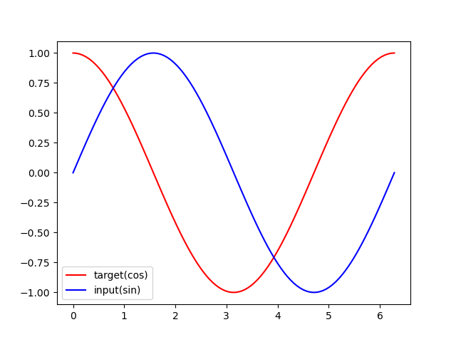
用 RNN 来及时预测时间序列
1、训练数据
用 sin 的曲线预测出 cos 的曲线
import torch
from torch import nn
import numpy as np
import matplotlib.pyplot as plt

torch.manual_seed(1)

# 超参数
TIME_STEP = 10      # rnn时间步长/图像高度
INPUT_SIZE = 1      # rnn输入大小/图像宽度
LR = 0.02           # 学习率

# 显示数据
steps = np.linspace(0, np.pi*2, 100, dtype=np.float32)  # float32 for converting torch FloatTensor
x_np = np.sin(steps)
y_np = np.cos(steps)
plt.plot(steps, y_np, 'r-', label = 'target(cos)')
plt.plot(steps, x_np, 'b-', label = 'input(sin)')
plt.legend(loc='best')
plt.show()
2、RNN网络
class RNN(nn.Module):
    def __init__(self):
        super(RNN, self).__init__()
        self.rnn = nn.RNN(   # 一个普通的RNN就能胜任
            input_size=INPUT_SIZE,
            hidden_size=32,
            num_layers=1,
            batch_first=True,
        )
        self.out = nn.Linear(32, 1)

    def forward(self, x, h_state):    # 因为 hidden state 是连续的, 所以我们要一直传递这一个 state
        # x (batch, time_step, input_size)
        # h_state (n_layers, batch, hidden_size)
        # r_out (batch, time_step, output_size)
        r_out, h_state = self.rnn(x, h_state)  # h_state 也要做为RNN的输入  这次具有时间序列特征
        outs = []  # 保存所有时间点的预测值
        for time_step in range(r_out.size(1)):  # 对每一个时间点计算 output
            outs.append(self.out(r_out[:, time_step, :]))
        return torch.stack(outs, dim=1), h_state

    # 其实熟悉RNN的朋友应该知道, forward过程中的对每个时间点求输出还有一招使得计算量比较小的.不过上面的内容主要是为了呈现
    # PyTorch在动态构图上的优势, 所以我用了一个for loop 来搭建那套输出系统.下面介绍一个替换方式.使用 reshape 的方式整批计算.
    # def forward(self, x, h_state):
    #     r_out, h_state = self.rnn(x, h_state)
    #     r_out = r_out.view(-1, 32)
    #     outs = self.out(r_out)
    #     return outs.view(-1, 32, TIME_STEP), h_state

rnn = RNN()
print(rnn)
"""
RNN(
  (rnn): RNN(1, 32, batch_first=True)
  (out): Linear(in_features=32, out_features=1, bias=True)
)
"""
3、训练
可以看出, 我们使用 x 作为输入的 sin 值, 然后 y 作为想要拟合的输出, cos 值. 因为他们两条曲线是存在某种关系的, 所以我们就能用 sin 来预测 cos. rnn 会理解他们的关系, 并用里面的参数分析出来这个时刻 sin 曲线上的点如何对应上 cos 曲线上的点.
optimizer = torch.optim.Adam(rnn.parameters(), lr=LR)   # optimize all rnn parameters
loss_func = nn.MSELoss()

h_state = None   # 要使用初始 hidden state, 可以设成 None

for step in range(100):
    start, end = step * np.pi, (step+1)*np.pi   # time steps
    # sin 预测 cos
    steps = np.linspace(start, end, TIME_STEP, dtype=np.float32, endpoint=False)  # float32 for converting torch FloatTensor
    x_np = np.sin(steps)    # float32 for converting torch FloatTensor
    y_np = np.cos(steps)

    # 原来只有一维的数据,利用np.newaxis,np.newaxis的作用就是在这一位置增加一个一维,这一位置指的是np.newaxis所在的位置
    x = torch.from_numpy(x_np[np.newaxis, :, np.newaxis])    # shape (batch, time_step, input_size)  (1,10,1)
    y = torch.from_numpy(y_np[np.newaxis, :, np.newaxis])

    prediction, h_state = rnn(x, h_state)   # rnn 对于每个 step 的 prediction, 还有最后一个 step 的 h_state
    # !!  下一步十分重要 !!
    h_state = h_state.data  # 要把 h_state 重新包装一下才能放入下一个 iteration, 不然会报错

    loss = loss_func(prediction, y)     # cross entropy loss
    optimizer.zero_grad()               # clear gradients for this training step
    loss.backward()                     # backpropagation, compute gradients
    optimizer.step()                    # apply gradients
    # plotting
    plt.plot(steps, y_np.flatten(), 'r-')
    plt.plot(steps, prediction.data.numpy().flatten(), 'b-')
    plt.draw(); plt.pause(0.05)

plt.ioff()
plt.show()
4、完整代码
import torch
from torch import nn
import numpy as np
import matplotlib.pyplot as plt

torch.manual_seed(1)

# 超参数
TIME_STEP = 10      # rnn时间步长/图像高度
INPUT_SIZE = 1      # rnn输入大小/图像宽度
LR = 0.02           # 学习率

# 显示数据
steps = np.linspace(0, np.pi*2, 100, dtype=np.float32)  # float32 for converting torch FloatTensor
x_np = np.sin(steps)
y_np = np.cos(steps)

# plt.plot(steps, y_np, 'r-', label = 'target(cos)')
# plt.plot(steps, x_np, 'b-', label = 'input(sin)')
# plt.legend(loc='best')
# plt.show()

class RNN(nn.Module):
    def __init__(self):
        super(RNN, self).__init__()
        self.rnn = nn.RNN(   # 一个普通的RNN就能胜任
            input_size=INPUT_SIZE,
            hidden_size=32,
            num_layers=1,
            batch_first=True,
        )
        self.out = nn.Linear(32, 1)

    def forward(self, x, h_state):    # 因为 hidden state 是连续的, 所以我们要一直传递这一个 state
        # x (batch, time_step, input_size)
        # h_state (n_layers, batch, hidden_size)
        # r_out (batch, time_step, output_size)
        r_out, h_state = self.rnn(x, h_state)  # h_state 也要做为RNN的输入  这次具有时间序列特征
        outs = []  # 保存所有时间点的预测值
        for time_step in range(r_out.size(1)):  # 对每一个时间点计算 output
            outs.append(self.out(r_out[:, time_step, :]))
        return torch.stack(outs, dim=1), h_state

    # 其实熟悉RNN的朋友应该知道, forward过程中的对每个时间点求输出还有一招使得计算量比较小的.不过上面的内容主要是为了呈现
    # PyTorch在动态构图上的优势, 所以我用了一个for loop 来搭建那套输出系统.下面介绍一个替换方式.使用 reshape 的方式整批计算.
    # def forward(self, x, h_state):
    #     r_out, h_state = self.rnn(x, h_state)
    #     r_out = r_out.view(-1, 32)
    #     outs = self.out(r_out)
    #     return outs.view(-1, 32, TIME_STEP), h_state

rnn = RNN()
print(rnn)
"""
RNN(
  (rnn): RNN(1, 32, batch_first=True)
  (out): Linear(in_features=32, out_features=1, bias=True)
)
"""

optimizer = torch.optim.Adam(rnn.parameters(), lr=LR)   # optimize all rnn parameters
loss_func = nn.MSELoss()

h_state = None   # 要使用初始 hidden state, 可以设成 None

for step in range(100):
    start, end = step * np.pi, (step+1)*np.pi   # time steps
    # sin 预测 cos
    steps = np.linspace(start, end, TIME_STEP, dtype=np.float32, endpoint=False)  # float32 for converting torch FloatTensor
    x_np = np.sin(steps)    # float32 for converting torch FloatTensor
    y_np = np.cos(steps)

    # 原来只有一维的数据,利用np.newaxis,np.newaxis的作用就是在这一位置增加一个一维,这一位置指的是np.newaxis所在的位置
    x = torch.from_numpy(x_np[np.newaxis, :, np.newaxis])    # shape (batch, time_step, input_size)  (1,10,1)
    y = torch.from_numpy(y_np[np.newaxis, :, np.newaxis])

    prediction, h_state = rnn(x, h_state)   # rnn 对于每个 step 的 prediction, 还有最后一个 step 的 h_state
    # !!  下一步十分重要 !!
    h_state = h_state.data  # 要把 h_state 重新包装一下才能放入下一个 iteration, 不然会报错

    loss = loss_func(prediction, y)     # cross entropy loss
    optimizer.zero_grad()               # clear gradients for this training step
    loss.backward()                     # backpropagation, compute gradients
    optimizer.step()                    # apply gradients
    # plotting
    plt.plot(steps, y_np.flatten(), 'r-')
    plt.plot(steps, prediction.data.numpy().flatten(), 'b-')
    plt.draw(); plt.pause(0.05)

plt.ioff()
plt.show()
十五、GAN生成对抗网络
https://mofanpy.com/tutorials/machine-learning/torch//intro-GAN/
https://mofanpy.com/tutorials/machine-learning/torch/GAN/
我的一句话介绍 GAN 就是: Generator 是新手画家, Discriminator 是新手鉴赏家, 你是高级鉴赏家. 你将著名画家的品和新手画家的作品都给新手鉴赏家评定, 并告诉新手鉴赏家哪些是新手画家画的, 哪些是著名画家画的, 新手鉴赏家就慢慢学习怎么区分新手画家和著名画家的画, 但是新手画家和新手鉴赏家是好朋友, 新手鉴赏家会告诉新手画家要怎么样画得更像著名画家, 新手画家就能将自己的突然来的灵感 (random noise) 画得更像著名画家。
下面是本节内容的效果, 绿线的变化是新手画家慢慢学习如何踏上画家之路的过程. 而能被认定为著名的画作在 upper bound 和 lower bound 之间.。
1、超参数设定
新手画家 (Generator) 在作画的时候需要有一些灵感 (random noise), 我们这些灵感的个数定义为 N_IDEAS. 而一幅画需要有一些规格, 我们将这幅画的画笔数定义一下, N_COMPONENTS 就是一条一元二次曲线(这幅画画)上的点个数. 为了进行批训练, 我们将一整批话的点都规定一下(PAINT_POINTS).
import torch
import torch.nn as nn
import numpy as np
import matplotlib.pyplot as plt

torch.manual_seed(1)
np.random.seed(1)

# 超参数
BATCH_SIZE = 64
LR_G = 0.0001
LR_D = 0.0001
N_IDEAS = 5 # think of this as number of ideas for generating an art work (Generator)
ART_COMPONENTS = 15   # 一条一元二次曲线(这幅画画)上的点个数 it could be total point G can draw in the canvas
PAINT_POINTS = np.vstack([np.linspace(-1,1,ART_COMPONENTS) for  _ in range(BATCH_SIZE)])
2、来自著名艺术家的绘画(真实目标)
def artist_works():   # 来自著名艺术家的绘画(真实目标)
    a = np.random.uniform(1, 2, size=BATCH_SIZE)[:, np.newaxis]
    paintings = a * np.power(PAINT_POINTS, 2) + (a-1)
    paintings = torch.from_numpy(paintings).float()
    return paintings
3、GAN网络
这里会创建两个神经网络, 分别是 Generator (新手画家), Discriminator(新手鉴赏家). G 会拿着自己的一些灵感当做输入, 输出一元二次曲线上的点 (G 的画).
D 会接收一幅画作 (一元二次曲线), 输出这幅画作到底是不是著名画家的画(是著名画家的画的概率).
G = nn.Sequential(                      # Generator
    nn.Linear(N_IDEAS, 128),            # random ideas (could from normal distribution)
    nn.ReLU(),
    nn.Linear(128, ART_COMPONENTS),     # making a painting from these random ideas
)

D = nn.Sequential(                      # Discriminator
    nn.Linear(ART_COMPONENTS, 128),     # receive art work either from the famous artist or a newbie like G
    nn.ReLU(),
    nn.Linear(128, 1),
    nn.Sigmoid(),                       # tell the probability that the art work is made by artist
)

opt_D = torch.optim.Adam(D.parameters(), lr=LR_D)
opt_G = torch.optim.Adam(G.parameters(), lr=LR_G)
# 有弹幕说 RMSprop 比较好
4、训练
接着我们来同时训练 D 和 G. 训练之前, 我们来看看G作画的原理. G 首先会有些灵感, G_ideas 就会拿到这些随机灵感 (可以是正态分布的随机数), 然后 G 会根据这些灵感画画. 接着我们拿着著名画家的画和 G 的画, 让 D 来判定这两批画作是著名画家画的概率
for step in range(10000):
    artist_paintings = artist_works()  # real painting from artist
    G_ideas = torch.randn(BATCH_SIZE, N_IDEAS, requires_grad=True)  # random ideas\n
    G_paintings = G(G_ideas)  # fake painting from G (random ideas)
    prob_artist1 = D(G_paintings)  # D try to reduce this prob
    G_loss = torch.mean(torch.log(1. - prob_artist1))
    opt_G.zero_grad()
    G_loss.backward()
    opt_G.step()

    prob_artist0 = D(artist_paintings)  # D try to increase this prob   D尝试增加这个概率
    prob_artist1 = D(G_paintings.detach())  # D try to reduce this prob D尝试减少这个概率
然后计算有多少来之画家的画猜对了, 有多少来自 G 的画猜对了, 我们想最大化这些猜对的次数. 这也就是 log(D(x)) + log(1-D(G(z)) 在论文中的形式. 而因为 torch 中提升参数的形式是最小化误差, 那我们把最大化 score 转换成最小化 loss, 在两个 score 的合的地方加一个符号就好. 而 G 的提升就是要减小 D 猜测 G 生成数据的正确率, 也就是减小 D_score1.
    D_loss = - torch.mean(torch.log(prob_artist0) + torch.log(1. - prob_artist1))
    G_loss = torch.mean(torch.log(1. - prob_artist1))
最后我们在根据 loss 提升神经网络就好了.
    opt_D.zero_grad()
    D_loss.backward(retain_graph=True)      # retain_graph 这个参数是为了再次使用计算图纸
    opt_D.step()

    opt_G.zero_grad()
    G_loss.backward()
    opt_G.step()
5、完整代码
import torch
import torch.nn as nn
import numpy as np
import matplotlib.pyplot as plt

torch.manual_seed(1)
np.random.seed(1)

# 超参数
BATCH_SIZE = 64
LR_G = 0.0001
LR_D = 0.0001
N_IDEAS = 5 # think of this as number of ideas for generating an art work (Generator)
ART_COMPONENTS = 15   # 一条一元二次曲线(这幅画画)上的点个数 it could be total point G can draw in the canvas
PAINT_POINTS = np.vstack([np.linspace(-1,1,ART_COMPONENTS) for  _ in range(BATCH_SIZE)])

# show our beautiful painting range
# plt.plot(PAINT_POINTS[0], 2 * np.power(PAINT_POINTS[0], 2) + 1, c='#74BCFF', lw=3, label='upper bound')
# plt.plot(PAINT_POINTS[0], 1 * np.power(PAINT_POINTS[0], 2) + 0, c='#FF9359', lw=3, label='lower bound')
# plt.legend(loc='upper right')
# plt.show()

def artist_works():   # 来自著名艺术家的绘画(真实目标)
    a = np.random.uniform(1, 2, size=BATCH_SIZE)[:, np.newaxis]
    paintings = a * np.power(PAINT_POINTS, 2) + (a-1)
    paintings = torch.from_numpy(paintings).float()
    return paintings


G = nn.Sequential(                      # Generator
    nn.Linear(N_IDEAS, 128),            # random ideas (could from normal distribution)
    nn.ReLU(),
    nn.Linear(128, ART_COMPONENTS),     # making a painting from these random ideas
)

D = nn.Sequential(                      # Discriminator
    nn.Linear(ART_COMPONENTS, 128),     # receive art work either from the famous artist or a newbie like G
    nn.ReLU(),
    nn.Linear(128, 1),
    nn.Sigmoid(),                       # tell the probability that the art work is made by artist
)

opt_D = torch.optim.Adam(D.parameters(), lr=LR_D)
opt_G = torch.optim.Adam(G.parameters(), lr=LR_G)
# 有弹幕说 RMSprop 比较好

plt.ion()

for step in range(10000):
    artist_paintings = artist_works()  # real painting from artist
    G_ideas = torch.randn(BATCH_SIZE, N_IDEAS, requires_grad=True)  # random ideas\n
    G_paintings = G(G_ideas)  # fake painting from G (random ideas)
    prob_artist1 = D(G_paintings)  # D try to reduce this prob
    G_loss = torch.mean(torch.log(1. - prob_artist1))
    opt_G.zero_grad()
    G_loss.backward()
    opt_G.step()

    prob_artist0 = D(artist_paintings)  # D try to increase this prob   D尝试增加这个概率
    prob_artist1 = D(G_paintings.detach())  # D try to reduce this prob D尝试减少这个概率
    D_loss = - torch.mean(torch.log(prob_artist0) + torch.log(1. - prob_artist1))
    opt_D.zero_grad()
    D_loss.backward(retain_graph=True)  # reusing computational graph
    opt_D.step()

    if step % 50 == 0:  # plotting
        plt.cla()
        plt.plot(PAINT_POINTS[0], G_paintings.data.numpy()[0], c='#4AD631', lw=3, label='Generated painting', )
        plt.plot(PAINT_POINTS[0], 2 * np.power(PAINT_POINTS[0], 2) + 1, c='#74BCFF', lw=3, label='upper bound')
        plt.plot(PAINT_POINTS[0], 1 * np.power(PAINT_POINTS[0], 2) + 0, c='#FF9359', lw=3, label='lower bound')
        plt.text(-.5, 2.3, 'D accuracy=%.2f (0.5 for D to converge)' % prob_artist0.data.numpy().mean(),
                 fontdict={'size': 13})
        plt.text(-.5, 2, 'D score= %.2f (-1.38 for G to converge)' % -D_loss.data.numpy(), fontdict={'size': 13})
        plt.ylim((0, 3));
        plt.legend(loc='upper right', fontsize=10);
        plt.draw();
        plt.pause(0.01)

plt.ioff()
plt.show()

十六、GPU 加速运算
import os
import torch
import torch.nn as nn
import torch.utils.data as Data
import torchvision      # 数据库模块

torch.manual_seed(1)    # reproducible

os.environ["CUDA_VISIBLE_DEVICES"] = "0"  # 使用编号为1,2号的GPU

# Hyper Parameters
EPOCH = 1           # 训练整批数据多少次, 为了节约时间, 我们只训练一次
BATCH_SIZE = 50
LR = 0.001          # 学习率
DOWNLOAD_MNIST = False  # 如果你已经下载好了mnist数据就写上 False

if not(os.path.exists('./mnist/')) or not os.listdir('./mnist/'):
    # not mnist dir or mnist is empyt dir
    DOWNLOAD_MNIST = True


# Mnist 手写数字
train_data = torchvision.datasets.MNIST(
    root='./mnist/',    # 保存或者提取位置
    train=True,  # this is training data
    transform=torchvision.transforms.ToTensor(),    # 转换 PIL.Image or numpy.ndarray 成
                                                    # torch.FloatTensor (C x H x W), 训练的时候 normalize 成 [0.0, 1.0] 区间
    download=DOWNLOAD_MNIST,          # 没下载就下载, 下载了就不用再下了
)

test_data = torchvision.datasets.MNIST(root='./mnist/', train=False)


# 批训练 50samples, 1 channel, 28x28 (50, 1, 28, 28)
train_loader = Data.DataLoader(dataset=train_data, batch_size=BATCH_SIZE, shuffle=True)

# 为了节约时间, 我们测试时只测试前2000个

# ############# 这里加cuda ###############
test_x = torch.unsqueeze(test_data.data, dim=1).type(torch.FloatTensor)[:2000].cuda()/255.   # shape from (2000, 28, 28) to (2000, 1, 28, 28), value in range(0,1)
test_y = test_data.targets[:2000].cuda()

# CNN模型搭建
class CNN(nn.Module):
    def __init__(self):
        super(CNN, self).__init__()
        self.conv1 = nn.Sequential(  # input shape (1,28,28)
            nn.Conv2d(
                in_channels=1,    # 输入高度
                out_channels=16,  # n_filters 输出高度
                kernel_size=5,    # 卷积核大小  filter size
                stride=1,         # 卷积核步进或者说步长,filter movement/step
                padding=2,        # 如果想要 con2d 出来的图片长宽没有变化, padding=(kernel_size-1)/2 当 stride=1

            ), ## output shape (16, 28, 28)
            nn.ReLU(),            # activation
            nn.MaxPool2d(kernel_size=2), #在2*2 空间里向下采样,output shape (16, 14, 14)
        )
        self.conv2 = nn.Sequential(   # input shape (16,14,14)
            nn.Conv2d(16,32,5,1,2),   # output shape(32,14,14)
            nn.ReLU(),
            nn.MaxPool2d(2),          # output size (32,7,7)
        )
        self.out = nn.Linear(32*7*7,10)  # 全连接层输出10个类

    def forward(self,x):
        x = self.conv1(x)
        x = self.conv2(x)
        x = x.view(x.size(0), -1) # 展平多维的卷积图成 (batch_size, 32 * 7 * 7)
        output = self.out(x)
        return output, x


def train_save():
    cnn = CNN()
    # ############# 这里加cuda ###############
    cnn.cuda()###将所有模型参数和缓冲区转移到GPU

    print(cnn)

    optimizer = torch.optim.Adam(cnn.parameters(), lr=LR) # 优化整一个CNN的参数
    loss_func = nn.CrossEntropyLoss()


    # training and testing
    for epoch in range(EPOCH):
        for step, (b_x, b_y) in enumerate(train_loader):   # gives batch data, normalize x when iterate train_loader
            # !!!!!!!! 这里有修改 !!!!!!!!! #
            b_x = b_x.cuda()   # Tensor on GPU
            b_y = b_y.cuda()   # Tensor on GPU

            output = cnn(b_x)[0]            # cnn output
            loss = loss_func(output, b_y)   # cross entropy loss
            optimizer.zero_grad()           # clear gradients for this training step
            loss.backward()                 # backpropagation, compute gradients
            optimizer.step()                # apply gradients

            if step % 50 == 0:
                test_output, last_layer = cnn(test_x)

                # !!!!!!!! 这里有修改 !!!!!!!!! #
                pred_y = torch.max(test_output, 1)[1].cuda().data   # 将操作放去 GPU
                accuracy =  torch.sum(pred_y == test_y).type(torch.FloatTensor) / test_y.size(0)
                print('Epoch: ', epoch, '| train loss: %.4f' % loss.data.cpu().numpy(), '| test accuracy: %.2f' % accuracy)


    torch.save(cnn, './mnist_net/cnn_classification_net.pkl')  # 保存整个网络
    torch.save(cnn.state_dict(), './mnist_net/cnn_classification_net_params.pkl')  # 只保存网络中的参数 (速度快, 占内存少)

    """
    ...
    Epoch:  0 | train loss: 0.0306 | test accuracy: 0.97
    Epoch:  0 | train loss: 0.0147 | test accuracy: 0.98
    Epoch:  0 | train loss: 0.0427 | test accuracy: 0.98
    Epoch:  0 | train loss: 0.0078 | test accuracy: 0.98
    """

    # print 10 predictions from test data
    test_output, _ = cnn(test_x[:10])

    # !!!!!!!! 这里有修改 !!!!!!!!! #
    pred_y = torch.max(test_output, 1)[1].cuda().data
    print(pred_y, 'prediction number')
    print(test_y[:10], 'real number')
    """
    [7 2 1 0 4 1 4 9 5 9] prediction number
    [7 2 1 0 4 1 4 9 5 9] real number
    """


# 这种方式将会提取整个神经网络, 网络大的时候可能会比较慢.
def restore_net():
    # restore entire net1 to net2
    net2 = torch.load('./mnist_net/cnn_classification_net.pkl')
    net2.cuda()
    test_output, _ = net2(test_x[:20])
    pred_y = torch.max(test_output, 1)[1].cuda().data
    print(pred_y, 'prediction number')
    print(test_y[:20], 'real number')

if __name__ == '__main__':
    GO_train = False
    if GO_train:
        train_save()
    else:
        restore_net()
本文作者:薄书
本文链接:https://www.cnblogs.com/aimoboshu/p/13846744.html
版权声明:本作品采用知识共享署名-非商业性使用-禁止演绎 2.5 中国大陆许可协议进行许可。


【推荐】国内首个AI IDE,深度理解中文开发场景,立即下载体验Trae
【推荐】编程新体验,更懂你的AI,立即体验豆包MarsCode编程助手
【推荐】抖音旗下AI助手豆包,你的智能百科全书,全免费不限次数
【推荐】轻量又高性能的 SSH 工具 IShell:AI 加持,快人一步