鸢尾花数据集的分类——SVM算法

Iris 鸢尾花数据集是一个经典数据集，在统计学习和机器学习领域都经常被用作示例。数据集内包含 3 类共 150 条记录，每类各 50 个数据，每条记录都有 4 项特征：花萼长度、花萼宽度、花瓣长度、花瓣宽度，可以通过这4个特征预测鸢尾花卉属于（iris-setosa, iris-versicolour, iris-virginica）三种中的哪一品种。

1、鸢尾花数据集的分类——SVM算法

#!/usr/bin/python
# -*- coding:utf-8 -*-

import numpy as np
from sklearn import svm
from sklearn.model_selection import train_test_split
import matplotlib as mpl
import matplotlib.pyplot as plt

def iris_type(s):
    it = {b'Iris-setosa': 0, b'Iris-versicolor': 1, b'Iris-virginica': 2}
    return it[s]


# 'sepal length', 'sepal width', 'petal length', 'petal width'
iris_feature = u'花萼长度', u'花萼宽度', u'花瓣长度', u'花瓣宽度'


def show_accuracy(a, b, tip):
    acc = a.ravel() == b.ravel()
    print (tip + '正确率：', np.mean(acc))


if __name__ == "__main__":
    path = 'iris.data'  # 数据文件路径)
    data = np.loadtxt(path, dtype=float, delimiter=',', converters={4: iris_type})
    x, y = np.split(data, (4,), axis=1)
    x = x[:, :2]
    x_train, x_test, y_train, y_test = train_test_split(x, y, random_state=1, train_size=0.6)

    # 分类器
    # clf = svm.SVC(C=0.1, kernel='linear', decision_function_shape='ovr')
    clf = svm.SVC(C=0.8, kernel='rbf', gamma=20, decision_function_shape='ovr')
    clf.fit(x_train, y_train.ravel())

    # 准确率
    print (clf.score(x_train, y_train))  # 精度
    y_hat = clf.predict(x_train)
    show_accuracy(y_hat, y_train, '训练集')
    print (clf.score(x_test, y_test))
    y_hat = clf.predict(x_test)
    show_accuracy(y_hat, y_test, '测试集')

    # 画图
    x1_min, x1_max = x[:, 0].min(), x[:, 0].max()  # 第0列的范围
    x2_min, x2_max = x[:, 1].min(), x[:, 1].max()  # 第1列的范围
    x1, x2 = np.mgrid[x1_min:x1_max:500j, x2_min:x2_max:500j]  # 生成网格采样点
    grid_test = np.stack((x1.flat, x2.flat), axis=1)  # 测试点

    Z = clf.decision_function(grid_test)    # 样本到决策面的距离
    print (Z)
    grid_hat = clf.predict(grid_test)       # 预测分类值
    print (grid_hat)
    grid_hat = grid_hat.reshape(x1.shape)  # 使之与输入的形状相同
    mpl.rcParams['font.sans-serif'] = [u'SimHei']  # 指定默认字体
    mpl.rcParams['axes.unicode_minus'] = False

    cm_light = mpl.colors.ListedColormap(['#A0FFA0', '#FFA0A0', '#A0A0FF'])
    cm_dark = mpl.colors.ListedColormap(['g', 'r', 'b'])
    x1_min, x1_max = x[:, 0].min(), x[:, 0].max()  # 第0列的范围
    x2_min, x2_max = x[:, 1].min(), x[:, 1].max()  # 第1列的范围
    x1, x2 = np.mgrid[x1_min:x1_max:500j, x2_min:x2_max:500j]  # 生成网格采样点
    grid_test = np.stack((x1.flat, x2.flat), axis=1)  # 测试点
    plt.pcolormesh(x1, x2, grid_hat, cmap=cm_light)

    plt.scatter(x[:, 0], x[:, 1], c=y[:,0], edgecolors='k', s=50, cmap=cm_dark)      # 样本
    plt.scatter(x_test[:, 0], x_test[:, 1], s=120, facecolors='none', zorder=10)     # 圈中测试集样本
    plt.xlabel(iris_feature[0], fontsize=13)
    plt.ylabel(iris_feature[1], fontsize=13)
    plt.xlim(x1_min, x1_max)
    plt.ylim(x2_min, x2_max)
    plt.title(u'鸢尾花SVM二特征分类', fontsize=15)
    plt.grid()
    plt.show()

2、运行结果

0.8666666666666667
训练集正确率： 0.8666666666666667
0.65
测试集正确率： 0.65
[[-0.02248787 2.04243623 0.98005163]
[-0.02092291 2.04165431 0.9792686 ]
[-0.01929329 2.04084007 0.97845322]
...
[-0.04903923 2.05568979 0.99334945]
[-0.04903923 2.05568979 0.99334945]
[-0.04903923 2.05568979 0.99334945]]
[1. 1. 1. ... 1. 1. 1.]

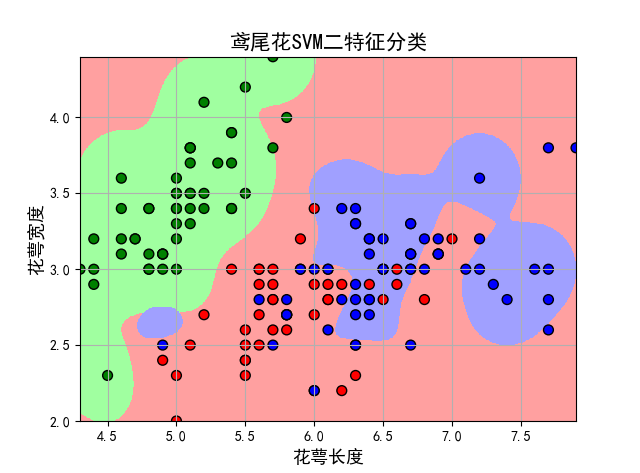
实验结果表明：采用SVM可以大概分类出这三种花卉，测试集精度为0.65。

3、补充说明

1）导入sklearn算法包

Scikit-Learn库已经实现了所有基本机器学习的算法，具体使用详见官方文档说明：http://scikit-learn.org/stable/auto_examples/index.html#support-vector-machines。

skleran中集成了许多算法，其导入包的方式如下所示：

支持向量机：from sklearn import svm

逻辑回归：from sklearn.linear_model import LogisticRegression

朴素贝叶斯：from sklearn.naive_bayes import GaussianNB

K-近邻：from sklearn.neighbors import KNeighborsClassifier

决策树：from sklearn.tree import DecisionTreeClassifier

2）使用numpy中的loadtxt读入数据文件

loadtxt()的使用方法：np.loadtxt(fpath, dtype, comments, delimiter, converters, skiprows, usecols)

fname:文件路径。eg：C:/Dataset/iris.txt。

dtype：数据类型。eg：float、str等。

delimiter：分隔符。eg：‘，’。

converters：将数据列与转换函数进行映射的字典。eg：{1:fun}，含义是将第2列对应转换函数进行转换。

usecols：选取数据的列。

通过loadtxt()函数中的converters参数将第五列通过转换函数iris_type(s)映射成浮点类型的数据。

3） 将Iris分为训练集与测试集

1. split(数据，分割位置，轴=1（水平分割） or 0（垂直分割）)。

2. x = x[:, :2]是为方便后期画图更直观，故只取了前两列特征值向量训练。

3. sklearn.model_selection.train_test_split随机划分训练集与测试集。train_test_split(train_data,train_target,test_size=数字, random_state=0)

参数解释：

train_data：所要划分的样本特征集

train_target：所要划分的样本结果

test_size：样本占比，如果是整数的话就是样本的数量

random_state：是随机数的种子。填1: 每次产生随机数组是一样的。但填0或不填，每次都会不一样。

4） 训练svm分类器

clf = svm.SVC(C=0.1, kernel='linear', decision_function_shape='ovr')

clf = svm.SVC(C=0.8, kernel='rbf', gamma=20, decision_function_shape='ovr')

clf.fit(x_train, y_train.ravel())

注：

kernel='linear'时，为线性核，C越大分类效果越好，但有可能会过拟合（defaul C=1）。

kernel='rbf'时（default），为高斯核，gamma值越小，分类界面越连续；gamma值越大，分类界面越“散”，分类效果越好，但有可能会过拟合。

decision_function_shape='ovr'时，为one v rest，即一个类别与其他类别进行划分，可实现多分类。

decision_function_shape='ovo'时，为one v one，即将类别两两之间进行划分，用二分类的方法模拟多分类的结果。

5） 作图

pcolormesh(x,y,z,cmap)这里参数代入x1，x2，grid_hat，cmap=cm_light绘制的是背景。

scatter中edgecolors是指描绘点的边缘色彩，s指描绘点的大小，cmap指点的颜色。

xlim指图的边界。

参考文献

[1]  https://www.cnblogs.com/luyaoblog/p/6775342.html

附录

数据集下载：

链接：https://pan.baidu.com/s/1fYNFUYNIXO8OrUiqlpKYqA
提取码：dfzw