第二讲 回归初心，方得始终--回归-----学习总结

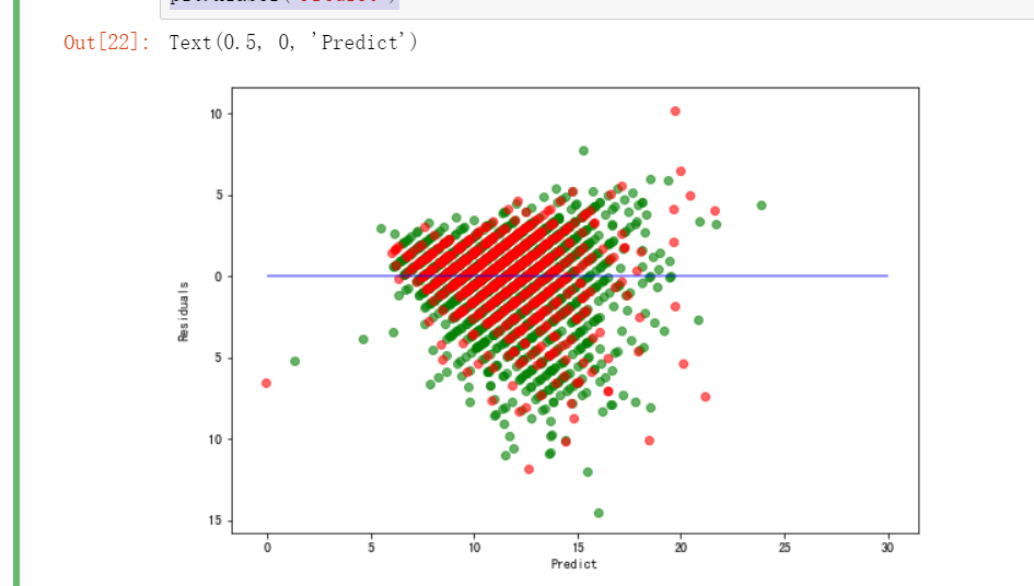
plt.figure(figsize=(9, 6))
y_train_pred_ridge = ridge.predict(X_train[features_without_ones])
plt.scatter(y_train_pred_ridge, y_train_pred_ridge - y_train, c="g", alpha=0.6)
plt.scatter(y_test_pred_ridge, y_test_pred_ridge - y_test, c="r",alpha=0.6)
plt.hlines(y=0, xmin=0, xmax=30,color="b",alpha=0.6)
plt.ylabel("Residuals")
plt.xlabel("Predict")

 

基于一份鲍鱼数据集，利用回归模型建立自动鲍鱼年龄预测模型。 使用 Python 实现线性回归和岭回归算法，并与 Sklearn 中的实现进行对比 借助 Sklearn 工具，对线性回归、岭回归和 LASSO 三种模型的预测效果使用 MAE 和决定系数进行效果评估 残差图和正则化路径对模型表现进行分析

鲍鱼是一种贝类，在世界许多地方被认为是美味佳肴。是铁和泛酸的极好来源，也是澳大利亚、美洲和东亚的营养食品资源和农业。100克鲍鱼就能给人体提供超过 20% 上述每日摄入营养素。鲍鱼的经济价值与年龄正相关。因此，准确检测鲍鱼的年龄对养殖户和消费者确定鲍鱼的价格具有重要意义。

然而，目前确定鲍鱼年龄的技术是相当昂贵和低效的。农场主通常把鲍鱼的壳割下来，用显微镜数鲍鱼环的数量，以估计鲍鱼的年龄。因此判断鲍鱼的年龄很困难，主要是因为鲍鱼的大小不仅取决于年龄，而且还取决于食物的供应情况。此外，鲍鱼有时会形成所谓的“发育不良”群体，这些群体的生长特性与其他鲍鱼种群有很大不同。这种复杂的方法增加了成本，限制了应用范围。本案例的目标是使用机器学习中的回归模型，找出最佳的指标来预测鲍鱼环数，进而预测鲍鱼的年龄。

1 数据集探索性分析

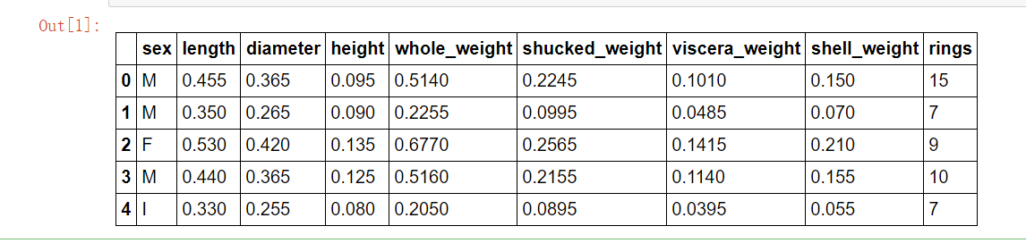
我们首先将鲍鱼数据集 abalone_dataset.csv 读取为 Pandas 的 DataFrame 格式。

import pandas as pd
import warnings
warnings.filterwarnings('ignore')
data = pd.read_csv("./input/abalone_dataset.csv")  #文件读取
data.head()

 

 查看数据集中样本数量和特征数量。

data.shape

 

 

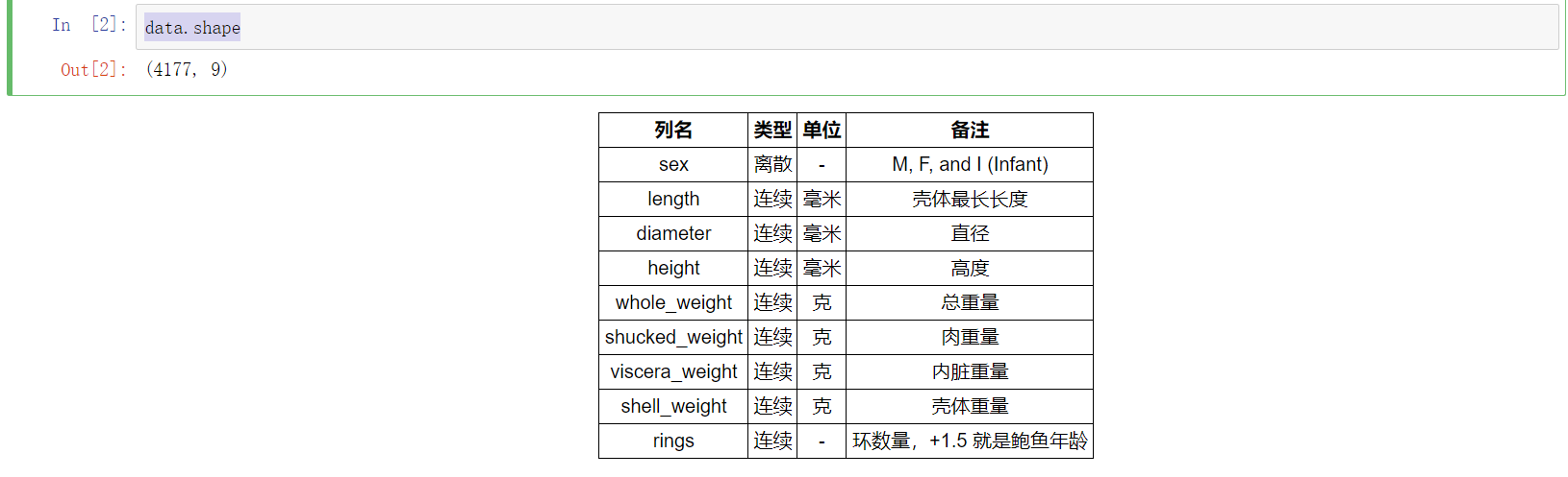
数据集一共有 4177 个样本，每个样本有 9 个特征。其中 rings 为鲍鱼环数，能够代表鲍鱼年龄，是预测变量。除了 sex 为离散特征，其余都为连续变量。

 

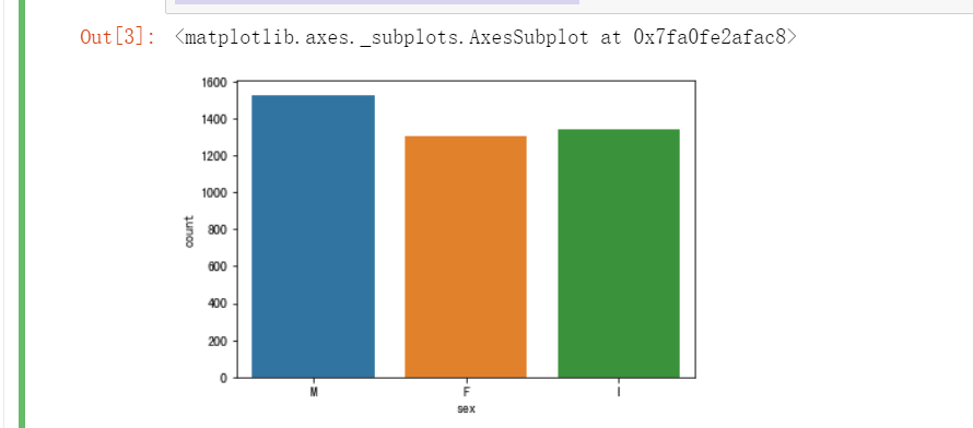
首先借助 seaborn 中的 countplot 函数绘制条形图，观察 sex 列的取值分布情况。

import seaborn as sns
import matplotlib.pyplot as plt
%matplotlib inline
sns.countplot(x = "sex", data = data)

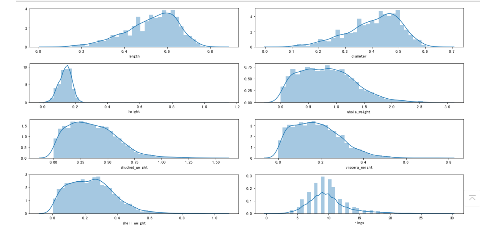
 对于连续特征，可以使用 seaborn 的 distplot 函数绘制直方图观察特征取值情况。我们将 8 个连续特征的直方图绘制在一个 4 行 2 列的子图布局中

i = 1 # 子图记数
plt.figure(figsize=(16, 8))     #figsize:指定figure的宽和高，单位为英寸；

for col in data.columns[1:]:
    plt.subplot(4,2,i)
    i = i + 1
    sns.distplot(data[col])  
plt.tight_layout()       #tight_layout会自动调整子图参数，使之填充整个图像区域

 

sns.pairplot(data,hue="sex")   #hue ：针对某一字段进行分类        可以看到对角线上是各个属性的直方图（分布图），而非对角线上是两个不同属性之间的相关图

<seaborn.axisgrid.PairGrid at 0x7f12a1086b00>

 

 

从以上连续特征之间的散点图我们可以看到一些基本的结果：

• 例如从第一行可以看到鲍鱼的长度 length 和鲍鱼直径 diameter 、鲍鱼高度 height 存在明显的线性关系。鲍鱼长度与鲍鱼的四种重量之间存在明显的非线性关系。

• 观察最后一行，鲍鱼环数 rings 与各个特征均存在正相关性，其中与 height 的线性关系最为直观。

• 观察对角线上的直方图，可以看到幼鲍鱼（sex 取值为“I”）在各个特征上的取值明显小于其他成年鲍鱼。而雄性鲍鱼（sex 取值为“M”）和雌性鲍鱼（sex 取值为“F”）各个特征取值分布没有明显的差异。

 

为了定量地分析特征之间的线性相关性，我们计算特征之间的相关系数矩阵，并借助热力图将相关性可视化。

corr_df = data.corr()    ##相关系数矩阵,即给出任意两款菜之间的相关系数
corr_df

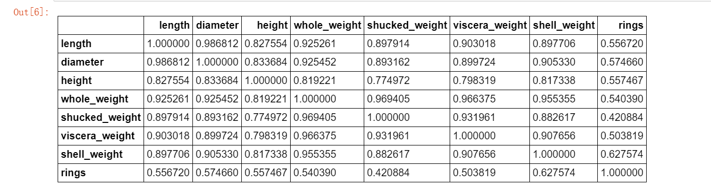
fig, ax = plt.subplots(figsize=(12, 12))
## 绘制热力图
ax = sns.heatmap(corr_df,linewidths=.5,cmap="Greens",annot=True,xticklabels=corr_df.columns, yticklabels=corr_df.index)
ax.xaxis.set_label_position('top') 
ax.xaxis.tick_top()

鲍鱼数据预处理

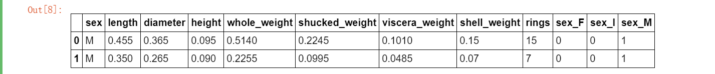
对 sex 特征进行 OneHot 编码

使用 Pandas 的 get_dummies 函数对 sex 特征做 OneHot 编码处理。

sex_onehot = pd.get_dummies(data["sex"], prefix="sex")
data[sex_onehot.columns] = sex_onehot
data.head(2)

 

 

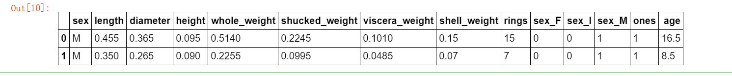
添加取值为 1 的特征

在后续实现线性回归模型时，需要使用设计矩阵 XX，其最后一列取值为 1 ，给数据添加一列 ones。

data["ones"] = 1
data.head(2)

 

 

根据鲍鱼环计算年龄

一般每过一年，鲍鱼就会在其壳上留下一道深深的印记，这叫生长纹，就相当于树木的年轮。在本数据集中，我们要预测的是鲍鱼的年龄，可以通过环数 rings 加上 1.5 得到。

data["age"] = data["rings"] + 1.5
data.head(2)

 

 

构造两组特征集

将预测目标设置为 age 列，然后构造两组特征，一组包含 ones，一组不包含 ones 。对于 sex 相关的列，我们只使用 sex_F 和 sex_M。

y = data["age"]
features_with_ones = ["length","diameter","height","whole_weight","shucked_weight","viscera_weight","shell_weight","sex_F","sex_M","ones"]
features_without_ones=["length","diameter","height","whole_weight","shucked_weight","viscera_weight","shell_weight","sex_F","sex_M"]
X = data[features_with_ones]

将鲍鱼数据集划分为训练集和测试集

将数据集随机划分为训练集和测试集，其中 80% 样本为训练集，剩余 20% 样本为测试集。

from sklearn import model_selection
X_train,X_test,y_train,y_test = model_selection.train_test_split(X,y,test_size=0.2, random_state=111)

实现线性回归和岭回归

使用 Numpy 实现线性回归

如果矩阵 XTXXTX 为满秩(行列式不为 0 )，则简单线性回归的解为 ŵ =(XTX)−1XTyw^=(XTX)−1XTy 。实现一个函数 linear_regression，其输入为训练集特征部分和标签部分，返回回归系数向量。 我们借助 numpy 工具中的 np.linalg.det 函数和 np.linalg.inv 函数分别求矩阵的行列式和矩阵的逆。

import numpy as np
def linear_regression(X,y):
    w = np.zeros_like(X.shape[1])
    if np.linalg.det(X.T.dot(X)) != 0 :
        w = np.linalg.inv(X.T.dot(X)).dot(X.T).dot(y)
    return w

使用上述实现的线性回归模型在鲍鱼训练集上训练模型。

w1 = linear_regression(X_train,y_train)
w1 = pd.DataFrame(data = w1,index = X.columns,columns = ["numpy_w"])
w1.round(decimals=2)

 

 

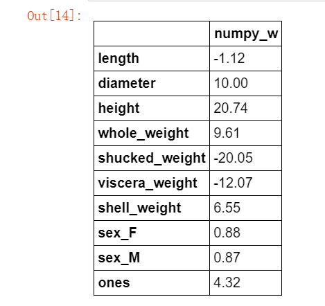
可见我们求得的模型为:

y=−−+1.12×length+10×diameter+20.74×height+9.61×whole_weight20.05×shucked_weight−12.07×viscera_weight+6.55×shell_weight0.88×sex_F+0.87×sex_M+4.32y=−1.12×length+10×diameter+20.74×height+9.61×whole_weight−20.05×shucked_weight−12.07×viscera_weight+6.55×shell_weight+0.88×sex_F+0.87×sex_M+4.32

 

 

sklearn 中的 linear_model 模块实现了常见的线性模型，包括线性回归、岭回归和 LASSO 等。对应的算法和类名如下表所示。

算法	类名
线性回归	linear_model.LinearRegression
岭回归	linear_model.Ridge
LASSO	linear_model.Lasso

下面我们使用 LinearRegression 构建线性回归模型。注意，此时传给 fit 方法的训练集的特征部分不包括 ones 列。模型训练完成后，lr.coef_ 属性和 lr.intercept_ 属性分别保存了学习到的回归系数向量和截距项。

from sklearn import linear_model
lr = linear_model.LinearRegression()
lr.fit(X_train[features_without_ones],y_train)
w_lr = []
w_lr.extend(lr.coef_)
w_lr.append(lr.intercept_)
w1["lr_sklearn_w"] = w_lr
w1.round(decimals=2)

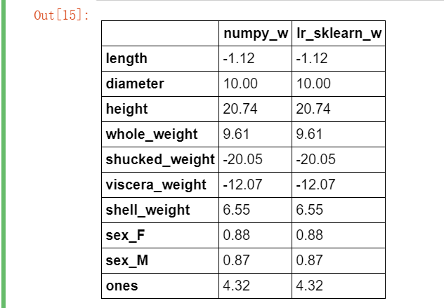
 对比上表可以看到，在训练集上训练鲍鱼年龄预测模型时，我们使用 Numpy 实现的线性回归模型与 sklearn 得到的结果是一致的。

 

使用 Numpy 实现岭回归 (Ridge)

 

def ridge_regression(X,y,ridge_lambda):
    penalty_matrix = np.eye(X.shape[1])
    penalty_matrix[X.shape[1] - 1][X.shape[1] - 1] = 0
    w = np.linalg.inv(X.T.dot(X) + ridge_lambda * penalty_matrix).dot(X.T).dot(y)
    return w

在鲍鱼训练集上使用 ridge_regression 函数训练岭回归模型，正则化系数设置为 1 。

w2 = ridge_regression(X_train,y_train,1.0)
w1["numpy_ridge_w"] = w2
w1.round(decimals=2)

 

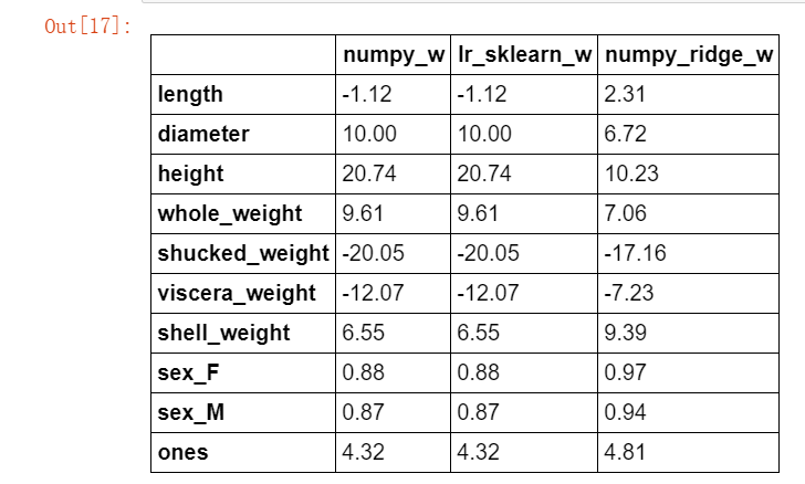
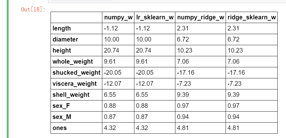
 与 sklearn 中岭回归对比，同样正则化系数设置为 1 。

from sklearn.linear_model import Ridge
ridge = linear_model.Ridge(alpha=1.0)
ridge.fit(X_train[features_without_ones],y_train)
w_ridge = []
w_ridge.extend(ridge.coef_)
w_ridge.append(ridge.intercept_)
w1["ridge_sklearn_w"] = w_ridge
w1.round(decimals=2)

 

 

使用 LASSO 构建鲍鱼年龄预测模型

from sklearn.linear_model import Lasso
lasso = linear_model.Lasso(alpha=0.01)
lasso.fit(X_train[features_without_ones],y_train)
print(lasso.coef_)
print(lasso.intercept_)

 

 

鲍鱼年龄预测模型效果评估

 

 

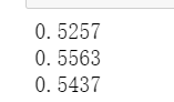
from sklearn.metrics import mean_squared_error
from sklearn.metrics import mean_absolute_error
y_test_pred_lr = lr.predict(X_test.iloc[:,:-1])
print(round(mean_absolute_error(y_test,y_test_pred_lr),4))

y_test_pred_ridge = ridge.predict(X_test[features_without_ones])
print(round(mean_absolute_error(y_test,y_test_pred_ridge),4))

y_test_pred_lasso = lasso.predict(X_test[features_without_ones])
print(round(mean_absolute_error(y_test,y_test_pred_lasso),4))

 

 

 

 

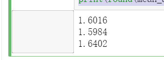
from sklearn.metrics import r2_score
print(round(r2_score(y_test,y_test_pred_lr),4))
print(round(r2_score(y_test,y_test_pred_ridge),4))
print(round(r2_score(y_test,y_test_pred_lasso),4))

 

 

 

残差图

残差图是一种用来诊断回归模型效果的图。在残差图中，如果点随机分布在0附近，则说明回归效果较好。 如果在残差图中发现了某种结构，则说明回归效果不佳，需要重新建模。

 

 

 

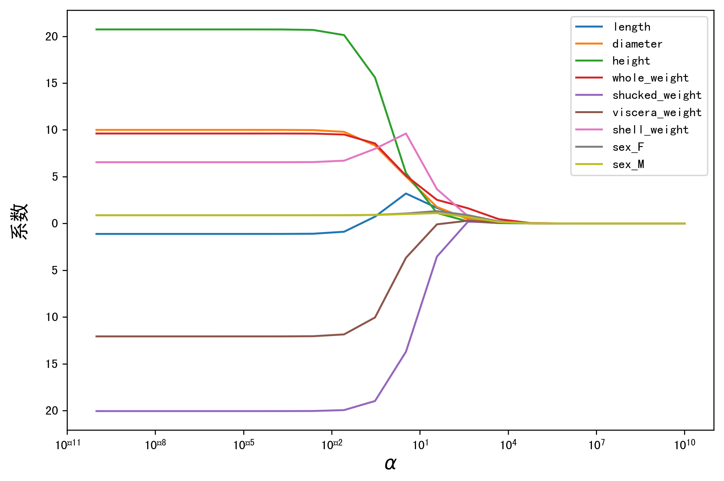
岭迹

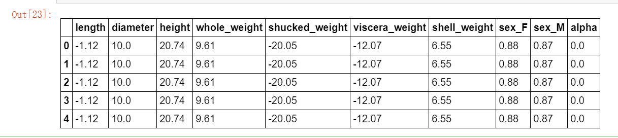
alphas = np.logspace(-10,10,20)
coef = pd.DataFrame()
for alpha in alphas:
    ridge_clf = Ridge(alpha=alpha)
    ridge_clf.fit(X_train[features_without_ones],y_train)
    df = pd.DataFrame([ridge_clf.coef_],columns=X_train[features_without_ones].columns)
    df['alpha'] = alpha
    coef = coef.append(df,ignore_index=True)
coef.head().round(decimals=2)

#绘图
plt.rcParams['figure.dpi'] = 300 #分辨率
plt.figure(figsize=(9, 6))
coef['alpha'] = coef['alpha']

for feature in X_train.columns[:-1]:
    plt.plot('alpha',feature,data=coef)
ax = plt.gca()
ax.set_xscale('log')
plt.legend(loc='upper right')
plt.xlabel(r'$\alpha$',fontsize=15)
plt.ylabel('系数',fontsize=15)

plt.show()

 

 

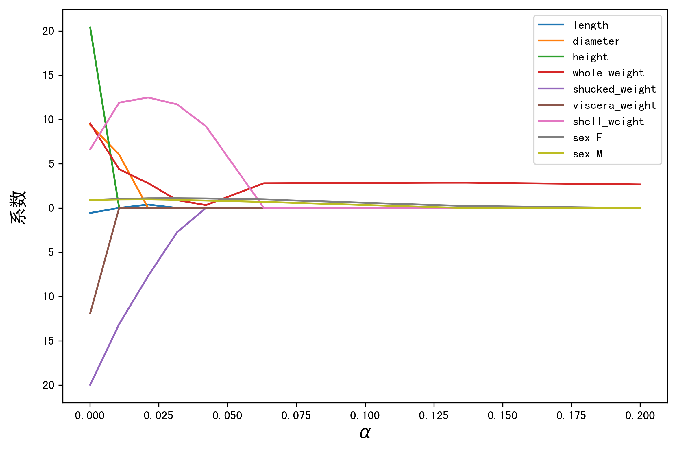
LASSO 的正则化路径

coef = pd.DataFrame()
for alpha in np.linspace(0.0001,0.2,20):
    lasso_clf = Lasso(alpha=alpha)
    lasso_clf.fit(X_train[features_without_ones],y_train)
    df = pd.DataFrame([lasso_clf.coef_],columns=X_train[features_without_ones].columns)
    df['alpha'] = alpha
    coef = coef.append(df,ignore_index=True)
coef.head()
#绘图
plt.figure(figsize=(9, 6))
for feature in X_train.columns[:-1]:
    plt.plot('alpha',feature,data=coef)
plt.legend(loc='upper right')
plt.xlabel(r'$\alpha$',fontsize=15)
plt.ylabel('系数',fontsize=15)
plt.show()

 

 

def ridge_regression(X,y,ridge_lambda):    penalty_matrix = np.eye(X.shape[1])    penalty_matrix[X.shape[1] - 1][X.shape[1] - 1] = 0    w = np.linalg.inv(X.T.dot(X) + ridge_lambda * penalty_matrix).dot(X.T).dot(y)    return w