
基于机器学习的自杀分析
背景
自杀是一项公认的全球性的重大社会问题和公共卫生问题,严重影响社会和经济的发展。据世界卫生组织估计,每年全世界有大约78.6万人自杀,其比例约为每年每10万人中有10.7人,也就是说每隔40秒就有人自杀。据联合国新闻,世卫组织发布的“2019年全球自杀状况”报告中的最新估计显示,自杀仍是全球主要死因之一。高收入国家的自杀率最高,美洲是唯一一个自杀率上升的地区。根据近年来世界各国的自杀率,可以发现:自杀率在性别上的差异在各国之间非常明显,一般的自杀率会男性高于女性,目前男性自杀率最高的国家为前苏联解体后的立陶宛、俄罗斯联邦、拉托维亚和爱沙尼亚等国家(年自杀率>60/10万),而女性自杀率最高的国家依次为斯里兰卡、中国、匈牙利和爱沙尼亚等(年自杀率>14/10万)。而在部分非洲和拉丁美洲国家自杀率却非常低,如埃及、秘鲁等(年自杀率<1/10万)。国际上习惯上将年自杀率>20/10万的国家称为高自杀率国家,年自杀率<10/10万的国家称为低自杀率国家,李振涛说,在1993年以前的统计中,中国属于低自杀率国家。 根据世界卫生组织在2019年发布的报告,全球每40秒钟就有一个人自杀身亡,自杀已经成为导致人类死亡的主要原因之一。一些国家的自杀人数增长迅速,甚至达60%。中国93%有自杀行为的人没有看过心理医生,在每年8万自杀未遂者中,被进行心理评估的还不到1%。中国的自杀防御工作缺乏一个全国性的计划来协调,政府机构对这一问题的重视不够,缺乏财力支持,也缺乏有效的评估心理因素的工具,更缺少高素质的研究人。
数据集来源
本次分析基于Kaggle数据集对自杀行文进行分析,探索自杀行为影响因素,并对自杀因素进行可视化,直观的表现影响自杀率的行为,并使用logistic回归、决策树、随机森林三种机器学习算法建立自杀行为分类模型,评估自杀结果,预测自杀率。
 1 import pandas as pd
 2 import numpy as np
 3 import matplotlib.pyplot as plt
 4 import seaborn as sns
 5 #import scikitplot as skplt
 6 import sklearn as sk
 7 from sklearn.model_selection import train_test_split
 8 from sklearn.preprocessing import StandardScaler
 9 plt.rcParams['font.sans-serif']='SimHei'
10 plt.rcParams['axes.unicode_minus']=False
11
12 import warnings
13 warnings.filterwarnings("ignore")
数据读取
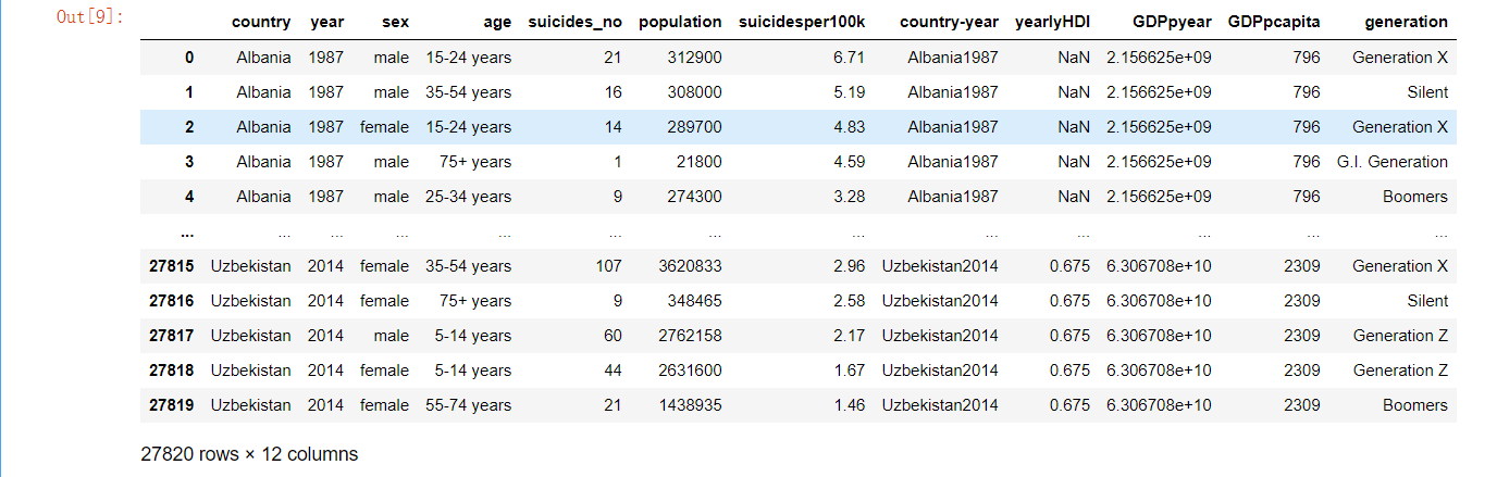
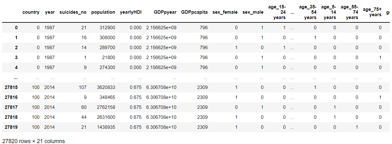
 1 # 导入原始自杀数据集并重新命名列:
 2 originaldata = pd.read_csv('./master.csv')
 3 # 国家,  年份,  性别,  年龄,  自杀人数,  人口数量,  自杀人数/总人口*100000(自杀率),
 4 # 国家-年份,     人类发展指数(用以衡量联合国各成员国经济社会发展水平的指标,是对传统的GNP指标挑战的结果。)
 5 # 年度国内生产总值(衡量经济发展的指标),      年人均国内生产总值:国内生产总值/人口 ,         世代
 6 originaldata.columns = ['country', 'year', 'sex', 'age', 'suicides_no', 'population','suicidesper100k',
 7                       'country-year', 'yearlyHDI',
 8                         'GDPpyear', 'GDPpcapita', 'generation']
 9
10 originaldata.head()

1 originaldata.shape

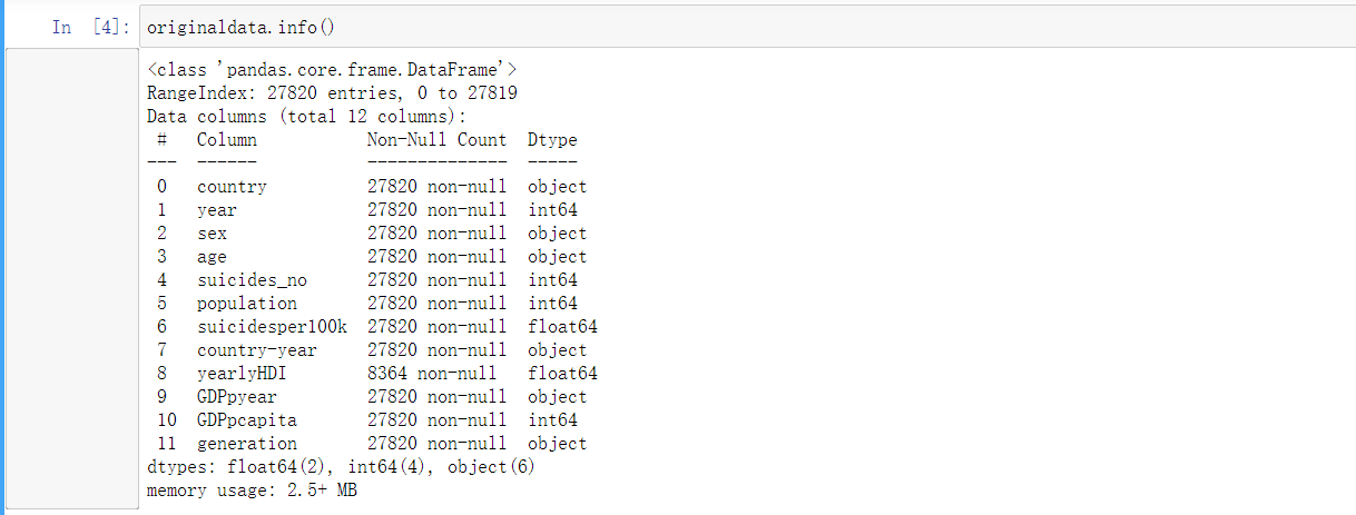
1 originaldata.info()
1 (originaldata=="male").sum()
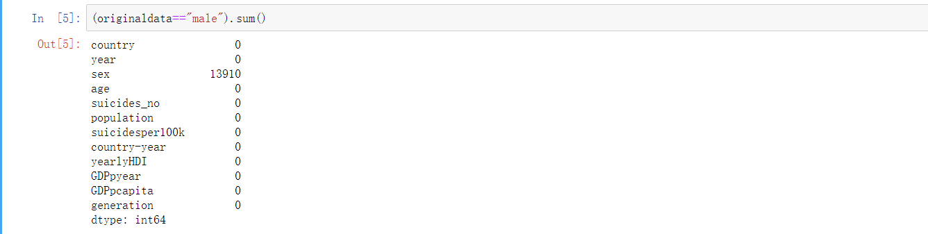
1 a = 13910/27820
2 a

1 df3 = originaldata.groupby("country").agg({"country":"count"})
2 df3.columns = ["count"]
3 df3

1 # 修复和清理原始数据
2 # 将 年度国内生产总值 数据中 ','分割去除掉(比如2,156,624,900),并且转换成float的数字类型
3 originaldata['GDPpyear'] = originaldata.apply(lambda x: float(x['GDPpyear'].replace(',', '')), axis=1)
4 originaldata['GDPpyear'].head(10)
5
6 # sex 转换为category类型
7 # Categoricals 是 pandas 的一种数据类型,对应着被统计的变量。Categoricals 是由固定的且有限数量的变量组成的。
8 originaldata.sex.astype('category')

1 df = originaldata.copy()#复制一份数据
2 df
1 df.suicidesper100k.mean()
2 df.suicidesper100k.std()
3 min(df.suicidesper100k)
4 max(df.suicidesper100k)

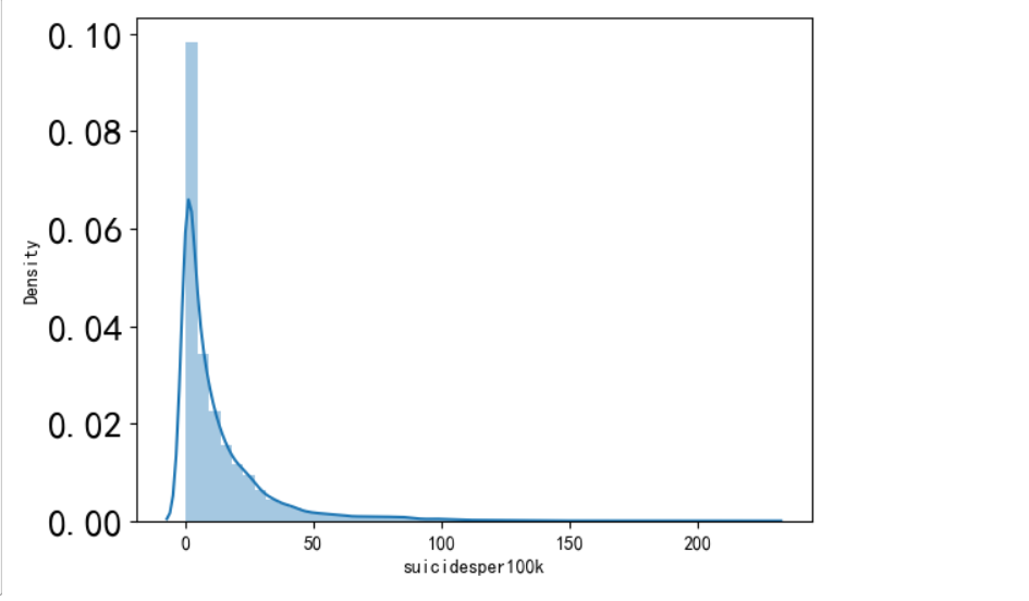
1 import seaborn as sns
2 sns.distplot(df.suicidesper100k)
3 plt.xticks(fontsize=10)
4 plt.yticks(fontsize=20)
5 plt.show()
探索性分析
 1 col = plt.cm.Spectral(np.linspace(0, 1, 20))
 2
 3 plt.figure(figsize=(8, 6))
 4 agedistf = pd.DataFrame(df.groupby('sex').get_group('female').groupby('age').suicides_no.sum())
 5 agedistm = pd.DataFrame(df.groupby('sex').get_group('male').groupby('age').suicides_no.sum())
 6 plt.bar(agedistm.index, agedistm.suicides_no, color=col[18])
 7 plt.bar(agedistf.index, agedistf.suicides_no, color=col[8])
 8 plt.legend(['male', 'female'], fontsize=16)
 9 plt.ylabel('Count', fontsize=14)
10 plt.xlabel('Suicides per 100K', fontsize=14)
11 plt.xticks(fontsize=10)
12 plt.yticks(fontsize=20)
13 plt.show()

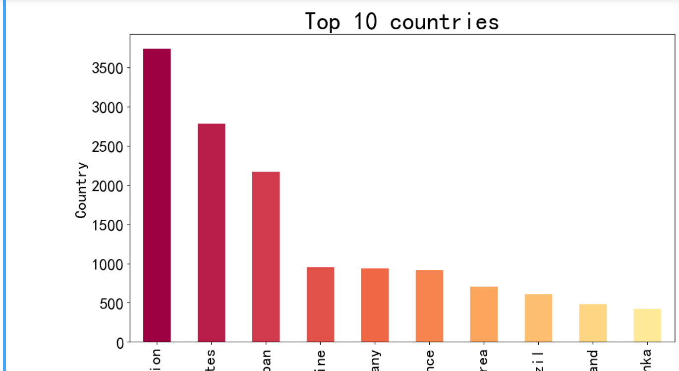
 1 col = plt.cm.Spectral(np.linspace(0, 1, 22))
 2 plt.figure(figsize=(12, 15))
 3
 4 plt.subplot(211)
 5 #自杀率(放大1000倍)的平均值最高的前10个国家
 6 df.groupby(['country']).suicidesper100k.mean().nlargest(10).plot(kind='bar', color=col, fontsize=20)
 7 plt.xlabel('Average Suicides/100k', size=20)
 8 plt.ylabel('Country', fontsize=20)
 9 plt.title('Top 10 countries', fontsize=30)
10
11 plt.figure(figsize=(12, 15))
12 plt.subplot(212)
13 #自杀人数的平均值最高的前10个国家
14 df.groupby(['country']).suicides_no.mean().nlargest(10).plot(kind='bar', color=col, fontsize=20)
15 plt.xlabel('Average Suicides_no', size=20)
16 plt.ylabel('Country', fontsize=20);
17 plt.title('Top 10 countries', fontsize=30)
18 plt.show()

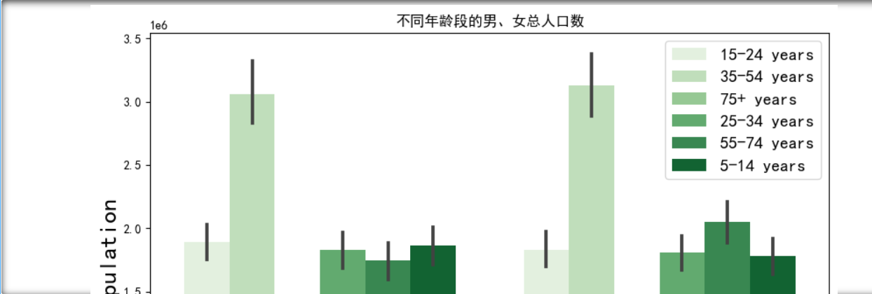
 1 plt.figure(figsize=(10, 16))
 2
 3 #总人口的各个年龄段的性别分布
 4 plt.subplot(311)
 5 sns.barplot(x='sex', y='population', hue='age', data=df, palette="Greens")  #hue按年龄分组
 6 plt.xticks(ha='right', fontsize=20)
 7 plt.ylabel('Population', fontsize=20)
 8 plt.xlabel('Sex', fontsize=20)
 9 plt.title("不同年龄段的男、女总人口数")
10 plt.legend(fontsize=14, loc='best')
11
12 #自杀人数的各个年龄段的性别分布
13 plt.subplot(312)
14 sns.barplot(x='sex', y='suicides_no', hue='age', data=df, palette="Greens")
15 plt.xticks(ha='right', fontsize=20)
16 plt.ylabel('suicides incidences', fontsize=20)
17 plt.xlabel('Sex', fontsize=20)
18 plt.title("不同年龄段的男、女自杀人口数")
19 plt.legend(fontsize=14)
20
21 #自杀率(放大1000倍)的各个年龄段的性别分布
22 plt.subplot(313)
23 sns.barplot(x='sex', y='suicidesper100k', hue='age', data=df,palette="Greens")
24 plt.xticks(ha='right', fontsize=20);
25 plt.ylabel('suicidesper100k',fontsize=20);
26 plt.xlabel('Sex',fontsize=20);
27 plt.title("不同年龄段的男、女自杀率")
28 plt.legend(fontsize=14);
29
30 plt.subplots_adjust(top=1.2)
31 plt.show()
 1 plt.figure(figsize=(12, 16))
 2
 3 # 具体按性别和年份 来看 男女的自杀率
 4 plt.subplot(311)
 5 sns.lineplot(x='year', y='suicidesper100k', hue='sex', data=df, palette="hot")  #hue按年龄分组
 6 plt.xticks(ha='right', fontsize=20)
 7 plt.ylabel('suicidesper100k', fontsize=20)
 8 plt.xlabel('year', fontsize=20)
 9 plt.legend(fontsize=14, loc='best')
10 plt.title("性别年份与自杀率关系图")
11 plt.show()

 1 plt.figure(figsize=(8, 6))
 2
 3 #选出year列并且去除重复的年份
 4 year = originaldata.groupby('year').year.unique()
 5
 6 #各个年份的自杀人数汇总
 7 #使用seaborn进行可视化,输入的数据必须为dataframe
 8 totalpyear = pd.DataFrame(originaldata.groupby('year').suicides_no.sum())
 9
10 plt.plot(year.index[0:31], totalpyear[0:31], color=col[18])  #选取范围为[0:31]  1985年到2015年
11 plt.xlabel('year', fontsize=15)
12 plt.ylabel('Total number of suicides in the world', fontsize=15)
13 plt.show()

 1 plt.figure(figsize=(20, 8))
 2
 3 # 自杀率(放大1000倍)的分布情况,y轴为个数
 4 plt.subplot(121)
 5 plt.hist(df.suicidesper100k, bins=30, color=col[18])   #bins:条形数
 6 plt.xlabel('Suicides per 100K of population', fontsize=25)
 7 plt.xticks(rotation = 0,                 fontsize = 20)
 8 plt.ylabel('count', fontsize=25)
 9 plt.yticks(                              fontsize = 20)
10
11 # 年人均国内生产总值的分布情况,y轴为个数
12 plt.subplot(122)
13 plt.hist(df.GDPpcapita, bins=30, color=col[7])
14 plt.xlabel('GDP', fontsize=25)
15 plt.xticks(rotation = 0,fontsize = 20)
16 plt.ylabel('count', fontsize=25)
17 plt.yticks(fontsize = 20)
18 plt.show()

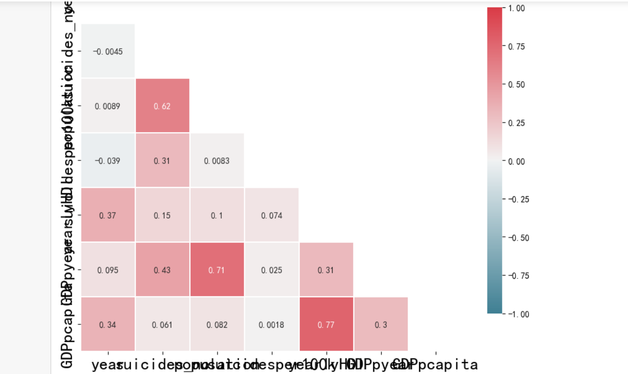
 1 corr = df.corr() #相关系数矩阵,即给出了任意两个变量之间的相关系数
 2
 3 # 相关矩阵的上三角部分与下三角对称。因此,热图不需要显示整个矩阵。在下一步隐藏上三角形。
 4 # 设置mask隐藏上三角
 5 # np.zeros_like() 返回一个零数组,其形状和类型与给定的数组相同。
 6 # 该 dtype=np.bool 参数会覆盖数据类型,因此我们的数组是一个布尔数组。
 7 # np.triu_indices_from(mask) 返回数组上三角形的索引。
 8 # 现在,我们将上三角形设置为True。 mask[np.triu_indices_from(mask)]= True
 9 mask = np.zeros_like(corr, dtype=np.bool)
10 mask[np.triu_indices_from(mask)] = True
11
12 # 在Seaborn中创建热图
13 f, ax = plt.subplots(figsize=(10, 8))
14 # 生成自定义发散颜色图
15 cmap = sns.diverging_palette(220, 10, as_cmap=True)
16
17 # 绘制热图
18 # 数据为 corr
19 # vmax,vmin:分别是热力图的颜色取值最大和最小范围
20 # center:数据表取值有差异时,设置热力图的色彩中心对齐值;通过设置center值,可以调整生成的图像颜色的整体深浅
21 # square:设置热力图矩阵小块形状,默认值是False
22 # linewidths(矩阵小块的间隔),
23 # cbar_kws:热力图侧边绘制颜色刻度条时,相关字体设置,默认值是None
24 sns.heatmap(corr, mask=mask, cmap=cmap, vmax=1, vmin=-1, center=0,
25             square=True, linewidths=0.2, cbar_kws={"shrink": 0.8},annot=True)
26 plt.xticks(fontsize=20)
27 plt.yticks(fontsize=20)
28 plt.show()
数据预处理
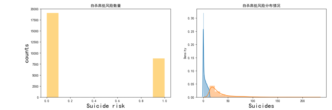
 1 #复制数据
 2 total = df.copy()
 3 # 对总人口用均值填充
 4 total.population.fillna(total.population.mean(), inplace=True)
 5 # 小于平均值的为低风险,大于平均值的为高风险
 6 total['risk'] = np.where(total.suicidesper100k < total.suicidesper100k.mean(), 0, 1)
 7
 8 plt.figure(figsize=(16, 5))
 9 plt.subplot(121)
10 plt.hist(total.risk, color=col[8])
11 plt.ylabel('counts', fontsize=20)
12 plt.xlabel('Suicide risk', fontsize=20)
13 plt.title("自杀高低风险数量")
14
15 plt.subplot(122)
16 sns.distplot(total.suicidesper100k[total.risk == 0], bins=10)
17 sns.distplot(total.suicidesper100k[total.risk == 1], bins=20)
18 plt.xlabel('Suicides', fontsize=20)
19 plt.title("自杀高低风险分布情况")
20 plt.show()
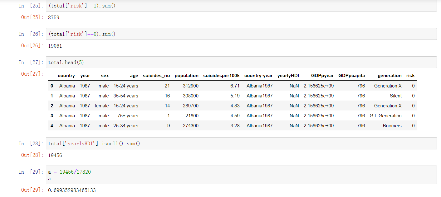
1 (total['risk']==1).sum()
2 (total['risk']==0).sum()
3 total.head(5)
4 total['yearlyHDI'].isnull().sum()
5 a = 19456/27820
6 a
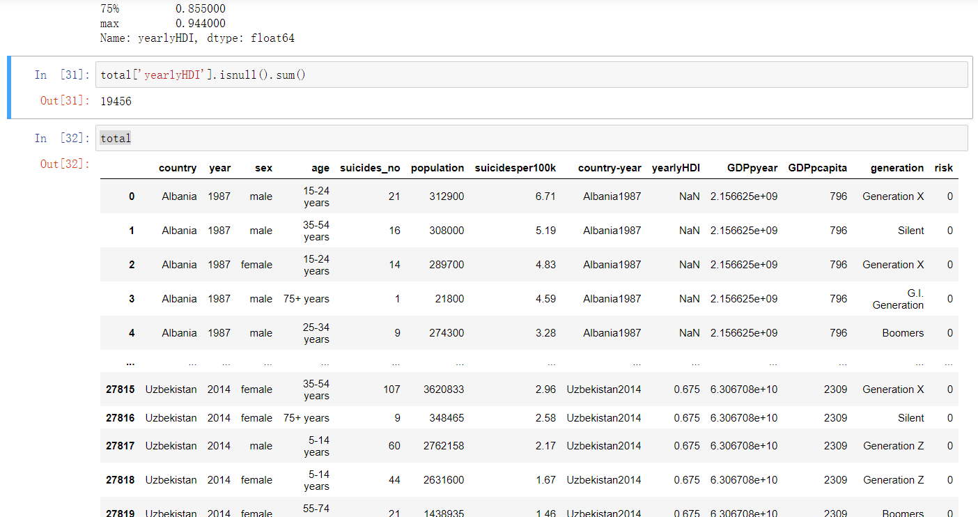
1 total['yearlyHDI'].describe()
2 total['yearlyHDI'].isnull().sum()
3 total
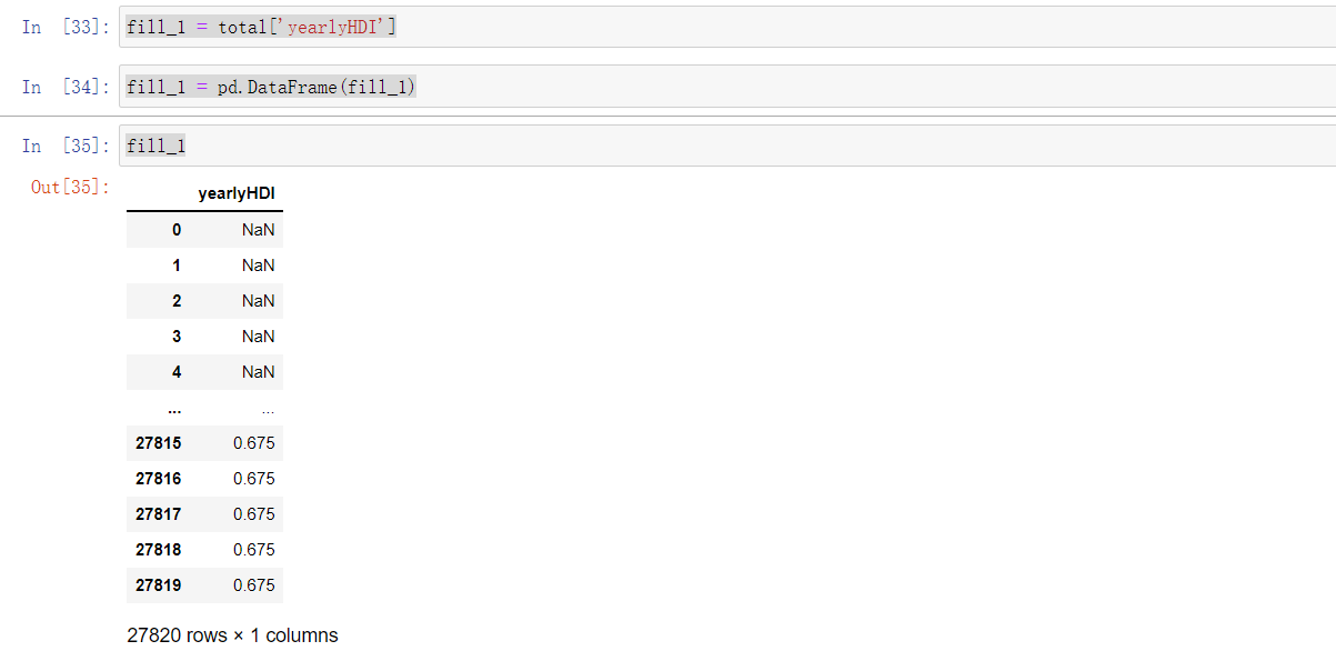
1 fill_1 = total['yearlyHDI']
2 fill_1 = pd.DataFrame(fill_1)
3 fill_1
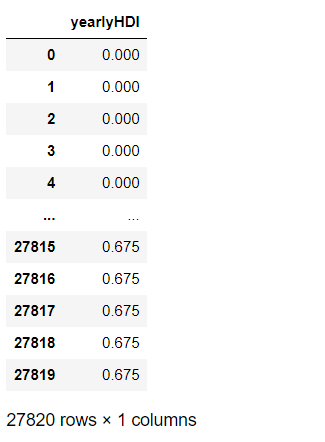
 1 from scipy.interpolate import lagrange #导入拉格朗日函数
 2 def ployinterp_column(s,n,k=2,result_type='broadcast'): # k=2表示用空值的前后两个数值来拟合曲线,从而预测空值
 3     y = s[list(range(n+2-k,n+2)) + list(range(n+3,n+3-k))] # 取值,range函数返回一个左闭右开([left,right))的序列数
 4     y = y[y.notnull()] # 取上一行中取出数值列表中的非空值,保证y的每行都有数值,便于拟合函数
 5     return lagrange(y.index,list(y))(n) # 调用拉格朗日函数,并添加索引
 6 for i in fill_1.columns: # 如果i在data的列名中,data.columns生成的是data的全部列名
 7     for j in range(len(fill_1)): # len(data)返回了data的长度,若此长度为5,则range(5)会产生从0开始计数的整数列表
 8         if (fill_1[i].isnull())[j]: # 如果data[i][j]为空,则调用函数ployinterp_column为其插值
 9             fill_1[i][j] = ployinterp_column(fill_1[i],j,result_type='broadcast')
10 fill_1
 1 # 对国家进行 标准化标签,将标签值统一转换成range(标签值个数-1)范围内
 2 # 相当于fit(X).transform(X),意思就是先进行fit(),进行数据拟合,然后在进行transform() 进行标准化处理
 3
 4 from sklearn.preprocessing import LabelEncoder
 5 le = LabelEncoder()
 6 total.country = le.fit_transform(total.country)
 7 total.country.unique()
 8
 9 # 为建立模型准备数据
10 X = total.drop(['suicidesper100k','risk','country-year'],axis = 1)
11 #用0进行填补
12 X['yearlyHDI'] = fill_1['yearlyHDI']
13 y = total['risk']
14 #对X进行独热编码处理
15 XS = pd.get_dummies(X)
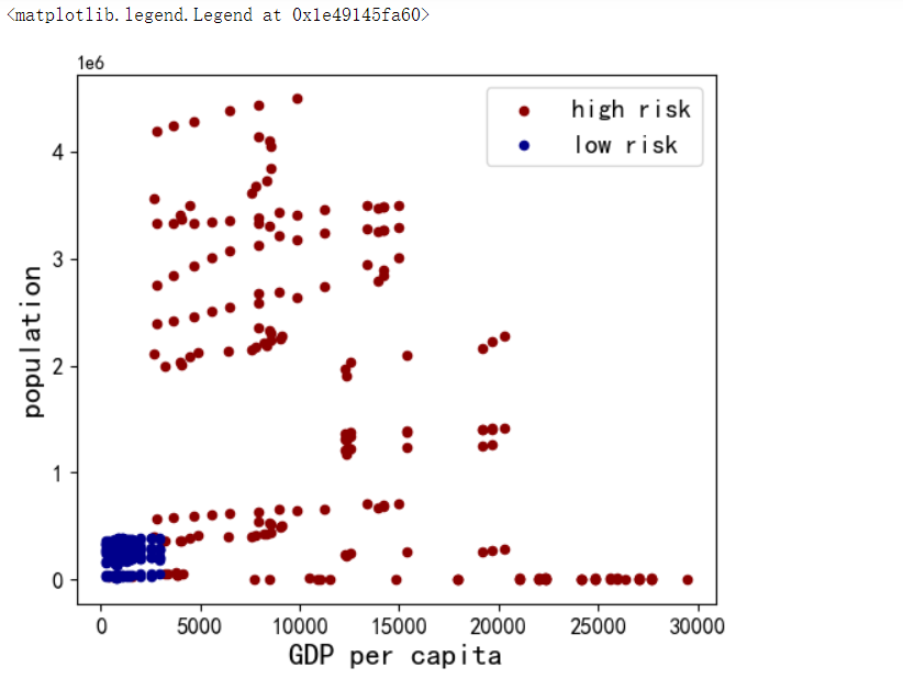
1 #GDP和人口的分布
2 ax1 = total[total['risk'] == 1][0:200].plot(kind='scatter', x='GDPpcapita', y='population', color='DarkRed',
3                                             label='high risk', figsize=(6, 5), fontsize=12)
4 total[total['risk'] == 0][0:200].plot(kind='scatter', x='GDPpcapita', y='population', color='DarkBlue',
5                                             label='low risk', ax=ax1)
6
7 plt.ylabel('population', fontsize=16)
8 plt.xlabel('GDP per capita', fontsize=16)
9 plt.legend(fontsize=14)
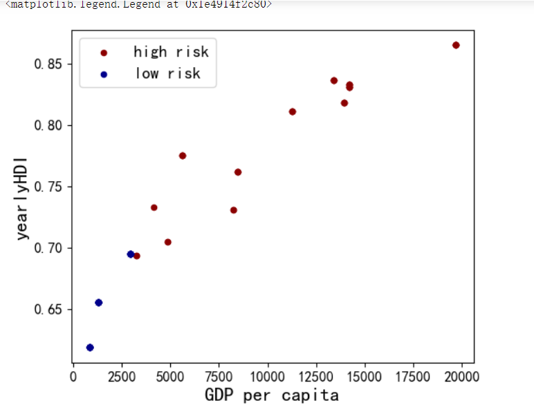
1 #GDP和人类发展指数的分布
2 ax1 = total[total['risk'] == 1][0:200].plot(kind='scatter', x='GDPpcapita', y='yearlyHDI', color='DarkRed',
3                                             label='high risk', figsize=(6, 5), fontsize=12)
4 total[total['risk'] == 0][0:200].plot(kind='scatter', x='GDPpcapita', y='yearlyHDI', color='DarkBlue',
5                                             label='low risk', ax=ax1)
6
7 plt.ylabel('yearlyHDI', fontsize=16)
8 plt.xlabel('GDP per capita', fontsize=16)
9 plt.legend(fontsize=14)
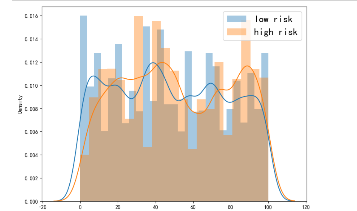
1 # 关于年份的高低自杀风险
2 fig = plt.figure(figsize=(30, 30))
3
4 plt.subplot(4, 3, 1)
5 sns.distplot(total[total.columns[0]][total.risk == 0], label='low risk')
6 sns.distplot(total[total.columns[0]][total.risk == 1], label='high risk')
7 plt.legend(loc='best', fontsize=18)
8 plt.xlabel(total.columns[0], fontsize=18)
9 plt.show()
建模
1 from sklearn.model_selection import train_test_split
2 # 将数据集拆分为训练集和测试集
3 # 首先将该数据3/4作为训练集,1/4作为测试集;再由训练集划分1/5作为验证集
4 X_train, X_test, y_train, y_test = train_test_split(XS, y, test_size=0.25, random_state=4)
5 X_train,X_valid,y_train,y_valid=train_test_split(X_train,y_train,test_size=0.2,random_state=4)
6 print('Train set:', X_train.shape, y_train.shape)
7 print('Test set:', X_test.shape, y_test.shape)
8 print('Test set:', X_valid.shape, y_valid.shape)

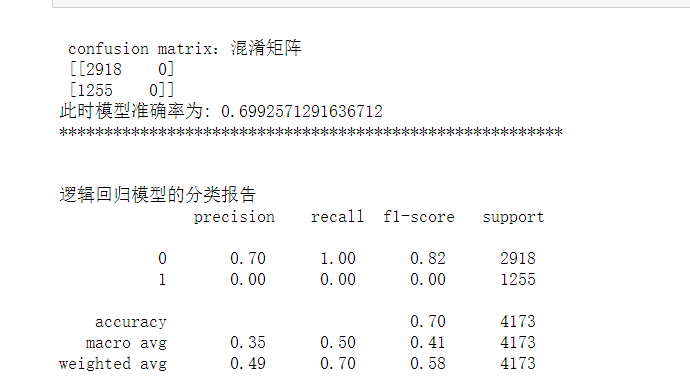
 1 from sklearn.linear_model import LogisticRegression
 2 from sklearn.metrics import recall_score,accuracy_score
 3 from sklearn.metrics import precision_recall_fscore_support
 4 from sklearn.metrics import confusion_matrix, classification_report
 5
 6 LR = LogisticRegression(C=0.001, solver='liblinear')
 7 LR.fit(X_train, y_train)
 8
 9 # 预测类别:0还是1
10 yLRhat = LR.predict(X_valid)
11
12 # 预测 0或1的概率(例如 [0.54689436, 0.45310564] 预测出来为0)
13 yLRhat_prob = LR.predict_proba(X_valid)
14
15 cm = confusion_matrix(y_valid, yLRhat)
16 print('\n confusion matrix:混淆矩阵 \n', cm)
17 print('此时模型准确率为:',accuracy_score(y_valid, yLRhat))
18 print('********************************************************')
19 print('\n')
20 print('逻辑回归模型的分类报告\n', classification_report(y_valid, yLRhat))
21 #skplt.metrics.plot_confusion_matrix(y_valid,yLRhat,normalize=True)
1 X_train.head()
 1 from sklearn.model_selection import GridSearchCV
 2
 3 param={"tol":[1e-4, 1e-3,1e-2], "C":[0.4, 0.6, 0.8]}
 4 grid = GridSearchCV(LogisticRegression(),param_grid=param, cv=5)#这里是5折交叉验证
 5 grid.fit(X_train,y_train)
 6 print(grid.best_params_)
 7 print(grid.best_score_)
 8
 9 #得到最好的逻辑回归分类器
10 best_LR=grid.best_estimator_
11
12 #进行训练、预测
13 best_LR.fit(X_train,y_train)
14 pred=best_LR.predict(X_valid)
15
16 cm = confusion_matrix(y_valid, pred)
17 print('\n confusion matrix:混淆矩阵 \n', cm)
18 print('最好的逻辑回归模型准确率为:',accuracy_score(y_valid, pred))
19 print('********************************************************')
20 print('\n')
21 print('最好的逻辑回归模型的分类报告\n', classification_report(y_valid, pred))

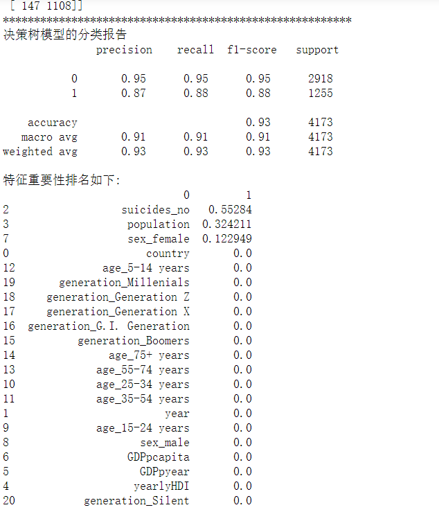
 1 from sklearn.tree import DecisionTreeClassifier
 2 from sklearn.metrics import accuracy_score
 3 from sklearn.metrics import confusion_matrix, classification_report
 4
 5 # 决策树学习
 6 # 函数为创建一个决策树模型
 7 # criterion:gini或者entropy,前者是基尼系数,后者是信息熵。
 8 # max_depth:  int or None, optional (default=None) 设置决策随机森林中的决策树的最大深度,深度越大,越容易过拟合,推荐树的深度为:5-20之间。
 9 # max_leaf_nodes: 通过限制最大叶子节点数,可以防止过拟合,默认是"None”,即不限制最大的叶子节点数。
10 DT = DecisionTreeClassifier(criterion="entropy", max_depth=7, max_leaf_nodes=30)
11 DT.fit(X_train, y_train)
12 ydthat = DT.predict(X_valid)
13
14 print('***决策树模型***')
15
16 #决策树模型性能评估
17 print('验证集上的准确率:', DT.score(X_valid, y_valid))
18 print('训练集上的准确率:', DT.score(X_train, y_train))
19
20 # 混淆矩阵
21 print('CM\n', confusion_matrix(y_valid, ydthat))
22 print('********************************************************')
23
24 print('决策树模型的分类报告\n', classification_report(y_valid, ydthat))
25
26 DTfeat_importance = DT.feature_importances_
27 DTfeat_importance = pd.DataFrame([X_train.columns, DT.feature_importances_]).T
28
29 # 特征重要性排序
30 print("特征重要性排名如下:")
31 print(DTfeat_importance.sort_values(by=1, ascending=False))
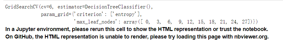
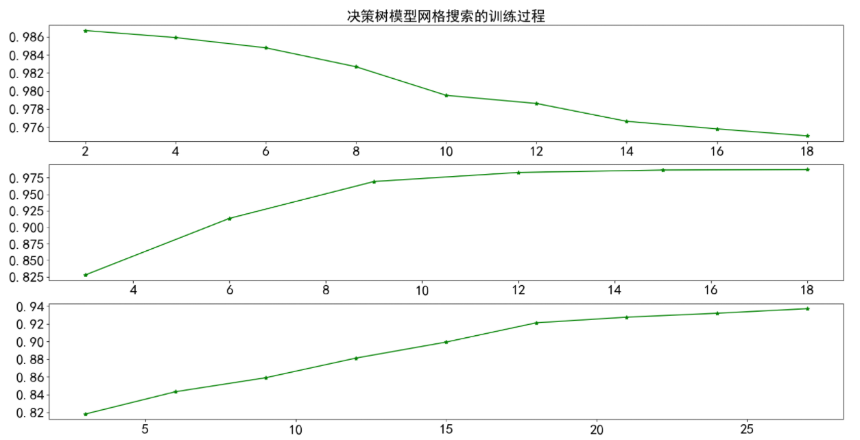
 1 # 通过cv_results观察过程并做图
 2 max_depth=np.arange(0,20,3)
 3 max_leaf_nodes=np.arange(0,30,3)
 4 min_samples_leaf =np.arange(0,20,2)
 5 param1= {'criterion':['entropy'],'max_depth':max_depth}
 6 param2= {'criterion':['entropy'],'min_samples_leaf':min_samples_leaf}
 7 param3= {'criterion':['entropy'],'max_leaf_nodes':max_leaf_nodes}
 8
 9
10 clf1 = GridSearchCV(DecisionTreeClassifier(),param_grid=param1,cv=6)
11 clf1.fit(X_train,y_train)
12
13 clf2 = GridSearchCV(DecisionTreeClassifier(),param_grid=param2,cv=6)
14 clf2.fit(X_train,y_train)
15
16
17 clf3 = GridSearchCV(DecisionTreeClassifier(),param_grid=param3,cv=6)
18 clf3.fit(X_train,y_train)
 1 fig = plt.figure(figsize=(20,10), dpi=100)
 2 ax = fig.add_subplot(311)
 3 ax.plot(min_samples_leaf,clf2.cv_results_['mean_test_score'],'g*-',)
 4 plt.title('决策树模型网格搜索的训练过程',fontsize=20)
 5 plt.xticks(fontsize=20)
 6 plt.yticks(fontsize=20)
 7
 8 ax = fig.add_subplot(312)
 9 ax.plot(max_depth,clf1.cv_results_['mean_test_score'],'g*-')
10 plt.xticks(fontsize=20)
11 plt.yticks(fontsize=20)
12 ax = fig.add_subplot(313)
13 ax.plot(max_leaf_nodes,clf3.cv_results_['mean_test_score'],'g*-')
14 plt.xticks(fontsize=20)
15 plt.yticks(fontsize=20)
16 plt.show()
 1 best_DT = DecisionTreeClassifier(criterion="entropy", max_depth=15, max_leaf_nodes=25,min_samples_leaf=2)
 2 best_DT.fit(X_train, y_train)
 3 ydthat =best_DT.predict(X_valid)
 4
 5 print('***决策树模型***')
 6
 7 #决策树模型性能评估
 8 print('验证集上的准确率:',best_DT.score(X_valid, y_valid))
 9 print('训练集上的准确率:',best_DT.score(X_train, y_train))
10
11 # 混淆矩阵
12 print('CM\n', confusion_matrix(y_valid, ydthat))
13 print('********************************************************')
14
15 print('决策树模型的分类报告\n', classification_report(y_valid, ydthat))
16
17 DTfeat_importance = best_DT.feature_importances_
18 DTfeat_importance = pd.DataFrame([X_train.columns, DT.feature_importances_]).T
19
20 # 特征重要性排序
21 print("特征重要性排名如下:")
22 print(DTfeat_importance.sort_values(by=1, ascending=False))

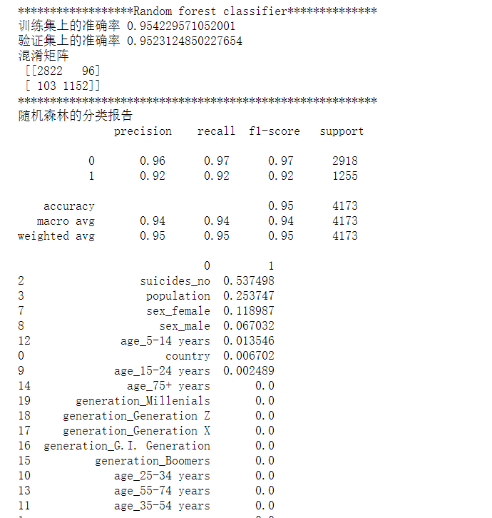
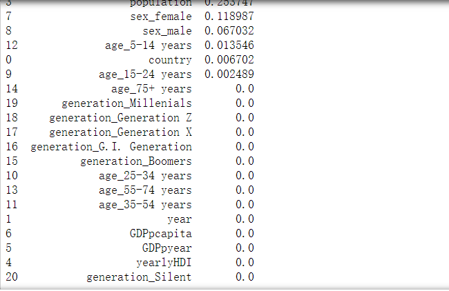
 1 # 随机森林可以视为多颗决策树的集成,鲁棒性更强,泛化能力更好,不易产生过拟合现象。但是噪声比较大的情况下会过拟合。
 2
 3 from sklearn.ensemble import RandomForestClassifier
 4
 5 random_forest = RandomForestClassifier(n_estimators=20, max_depth=10, min_samples_split=2, min_samples_leaf=5,
 6                                        max_leaf_nodes=20, max_features=len(X_train.columns))
 7
 8 random_forest.fit(X_train, y_train)
 9
10 yrfhat = random_forest.predict(X_valid)
11 feat_importance = random_forest.feature_importances_
12 rffeat_importance = pd.DataFrame([X_train.columns, random_forest.feature_importances_]).T
13
14 print('******************Random forest classifier**************')
15 print('训练集上的准确率', random_forest.score(X_train, y_train))
16 print('验证集上的准确率', random_forest.score(X_valid,y_valid))
17 print('混淆矩阵\n', confusion_matrix(y_valid, yrfhat))
18 print('********************************************************')
19 print('随机森林的分类报告\n', classification_report(y_valid, yrfhat))
20 print(rffeat_importance.sort_values(by=1, ascending=False))
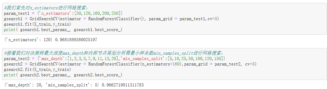
 1 #我们首先对n_estimators进行网格搜索:
 2 param_test1 = {'n_estimators':[50,120,160,200,250]}
 3 gsearch1 = GridSearchCV(estimator = RandomForestClassifier(), param_grid = param_test1,cv=5)
 4 gsearch1.fit(X_train,y_train)
 5 print( gsearch1.best_params_, gsearch1.best_score_)
 6 #接着我们对决策树最大深度max_depth和内部节点再划分所需最小样本数min_samples_split进行网格搜索。
 7 param_test2 = {'max_depth':[1,2,3,5,7,9,11,13,20],'min_samples_split':[5,10,25,50,100,120,150]}
 8 gsearch2 = GridSearchCV(estimator = RandomForestClassifier(n_estimators=160),param_grid = param_test2, cv=5)
 9 gsearch2.fit(X_train,y_train)
10 print( gsearch2.best_params_, gsearch2.best_score_)
 1 #最好的随机森林模型
 2 best_rf=RandomForestClassifier(n_estimators=160, max_depth=20, min_samples_split=5)
 3
 4 best_rf .fit(X_train, y_train)
 5
 6 yrfhat = best_rf .predict(X_valid)
 7 feat_importance = best_rf.feature_importances_
 8 rffeat_importance = pd.DataFrame([X_train.columns, random_forest.feature_importances_]).T
 9
10 print('******************随机森林模型**************')
11 print('训练集上的准确率',best_rf.score(X_train, y_train))
12 print('验证集上的准确率',best_rf.score(X_valid,y_valid))
13 print('混淆矩阵\n', confusion_matrix(y_valid, yrfhat))
14 print('********************************************************')
15 print('最好的随机森林模型的分类报告\n', classification_report(y_valid, yrfhat))
16 print(rffeat_importance.sort_values(by=1, ascending=False))

全代码附上
  1 import pandas as pd
  2 import numpy as np
  3 import matplotlib.pyplot as plt
  4 import seaborn as sns
  5 #import scikitplot as skplt
  6 import sklearn as sk
  7 from sklearn.model_selection import train_test_split
  8 from sklearn.preprocessing import StandardScaler
  9 plt.rcParams['font.sans-serif']='SimHei'
 10 plt.rcParams['axes.unicode_minus']=False
 11
 12 import warnings
 13 warnings.filterwarnings("ignore")
 14 # 导入原始自杀数据集并重新命名列:
 15 originaldata = pd.read_csv('./master.csv')
 16 # 国家,  年份,  性别,  年龄,  自杀人数,  人口数量,  自杀人数/总人口*100000(自杀率),
 17 # 国家-年份,     人类发展指数(用以衡量联合国各成员国经济社会发展水平的指标,是对传统的GNP指标挑战的结果。)
 18 # 年度国内生产总值(衡量经济发展的指标),      年人均国内生产总值:国内生产总值/人口 ,         世代
 19 originaldata.columns = ['country', 'year', 'sex', 'age', 'suicides_no', 'population','suicidesper100k',
 20                       'country-year', 'yearlyHDI',
 21                         'GDPpyear', 'GDPpcapita', 'generation']
 22
 23 originaldata.head()
 24 originaldata.shape
 25 originaldata.info()
 26 (originaldata=="male").sum()
 27 a = 13910/27820
 28 a
 29 df3 = originaldata.groupby("country").agg({"country":"count"})
 30 df3.columns = ["count"]
 31 df3
 32 # 修复和清理原始数据
 33 # 将 年度国内生产总值 数据中 ','分割去除掉(比如2,156,624,900),并且转换成float的数字类型
 34 originaldata['GDPpyear'] = originaldata.apply(lambda x: float(x['GDPpyear'].replace(',', '')), axis=1)
 35 originaldata['GDPpyear'].head(10)
 36
 37 # sex 转换为category类型
 38 # Categoricals 是 pandas 的一种数据类型,对应着被统计的变量。Categoricals 是由固定的且有限数量的变量组成的。
 39 originaldata.sex.astype('category')
 40 df = originaldata.copy()#复制一份数据
 41 df
 42 df.suicidesper100k.mean()
 43 df.suicidesper100k.std()
 44 min(df.suicidesper100k)
 45 max(df.suicidesper100k)
 46 import seaborn as sns
 47 sns.distplot(df.suicidesper100k)
 48 plt.xticks(fontsize=10)
 49 plt.yticks(fontsize=20)
 50 plt.show()
 51 df.suicidesper100k.isnull().sum()
 52 col = plt.cm.Spectral(np.linspace(0, 1, 20))
 53
 54 plt.figure(figsize=(8, 6))
 55 agedistf = pd.DataFrame(df.groupby('sex').get_group('female').groupby('age').suicides_no.sum())
 56 agedistm = pd.DataFrame(df.groupby('sex').get_group('male').groupby('age').suicides_no.sum())
 57 plt.bar(agedistm.index, agedistm.suicides_no, color=col[18])
 58 plt.bar(agedistf.index, agedistf.suicides_no, color=col[8])
 59 plt.legend(['male', 'female'], fontsize=16)
 60 plt.ylabel('Count', fontsize=14)
 61 plt.xlabel('Suicides per 100K', fontsize=14)
 62 plt.xticks(fontsize=10)
 63 plt.yticks(fontsize=20)
 64 plt.show()
 65 col = plt.cm.Spectral(np.linspace(0, 1, 22))
 66 plt.figure(figsize=(12, 15))
 67
 68 plt.subplot(211)
 69 #自杀率(放大1000倍)的平均值最高的前10个国家
 70 df.groupby(['country']).suicidesper100k.mean().nlargest(10).plot(kind='bar', color=col, fontsize=20)
 71 plt.xlabel('Average Suicides/100k', size=20)
 72 plt.ylabel('Country', fontsize=20)
 73 plt.title('Top 10 countries', fontsize=30)
 74
 75 plt.figure(figsize=(12, 15))
 76 plt.subplot(212)
 77 #自杀人数的平均值最高的前10个国家
 78 df.groupby(['country']).suicides_no.mean().nlargest(10).plot(kind='bar', color=col, fontsize=20)
 79 plt.xlabel('Average Suicides_no', size=20)
 80 plt.ylabel('Country', fontsize=20);
 81 plt.title('Top 10 countries', fontsize=30)
 82 plt.show()
 83 plt.figure(figsize=(10, 16))
 84
 85 #总人口的各个年龄段的性别分布
 86 plt.subplot(311)
 87 sns.barplot(x='sex', y='population', hue='age', data=df, palette="Greens")  #hue按年龄分组
 88 plt.xticks(ha='right', fontsize=20)
 89 plt.ylabel('Population', fontsize=20)
 90 plt.xlabel('Sex', fontsize=20)
 91 plt.title("不同年龄段的男、女总人口数")
 92 plt.legend(fontsize=14, loc='best')
 93
 94 #自杀人数的各个年龄段的性别分布
 95 plt.subplot(312)
 96 sns.barplot(x='sex', y='suicides_no', hue='age', data=df, palette="Greens")
 97 plt.xticks(ha='right', fontsize=20)
 98 plt.ylabel('suicides incidences', fontsize=20)
 99 plt.xlabel('Sex', fontsize=20)
100 plt.title("不同年龄段的男、女自杀人口数")
101 plt.legend(fontsize=14)
102
103 #自杀率(放大1000倍)的各个年龄段的性别分布
104 plt.subplot(313)
105 sns.barplot(x='sex', y='suicidesper100k', hue='age', data=df,palette="Greens")
106 plt.xticks(ha='right', fontsize=20);
107 plt.ylabel('suicidesper100k',fontsize=20);
108 plt.xlabel('Sex',fontsize=20);
109 plt.title("不同年龄段的男、女自杀率")
110 plt.legend(fontsize=14);
111
112 plt.subplots_adjust(top=1.2)
113 plt.show()
114 plt.figure(figsize=(12, 16))
115
116 # 具体按性别和年份 来看 男女的自杀率
117 plt.subplot(311)
118 sns.lineplot(x='year', y='suicidesper100k', hue='sex', data=df, palette="hot")  #hue按年龄分组
119 plt.xticks(ha='right', fontsize=20)
120 plt.ylabel('suicidesper100k', fontsize=20)
121 plt.xlabel('year', fontsize=20)
122 plt.legend(fontsize=14, loc='best')
123 plt.title("性别年份与自杀率关系图")
124 plt.show()
125 plt.figure(figsize=(8, 6))
126
127 #选出year列并且去除重复的年份
128 year = originaldata.groupby('year').year.unique()
129
130 #各个年份的自杀人数汇总
131 #使用seaborn进行可视化,输入的数据必须为dataframe
132 totalpyear = pd.DataFrame(originaldata.groupby('year').suicides_no.sum())
133
134 plt.plot(year.index[0:31], totalpyear[0:31], color=col[18])  #选取范围为[0:31]  1985年到2015年
135 plt.xlabel('year', fontsize=15)
136 plt.ylabel('Total number of suicides in the world', fontsize=15)
137 plt.show()
138 plt.figure(figsize=(20, 8))
139
140 # 自杀率(放大1000倍)的分布情况,y轴为个数
141 plt.subplot(121)
142 plt.hist(df.suicidesper100k, bins=30, color=col[18])   #bins:条形数
143 plt.xlabel('Suicides per 100K of population', fontsize=25)
144 plt.xticks(rotation = 0,                 fontsize = 20)
145 plt.ylabel('count', fontsize=25)
146 plt.yticks(                              fontsize = 20)
147
148 # 年人均国内生产总值的分布情况,y轴为个数
149 plt.subplot(122)
150 plt.hist(df.GDPpcapita, bins=30, color=col[7])
151 plt.xlabel('GDP', fontsize=25)
152 plt.xticks(rotation = 0,fontsize = 20)
153 plt.ylabel('count', fontsize=25)
154 plt.yticks(fontsize = 20)
155 plt.show()
156 corr = df.corr() #相关系数矩阵,即给出了任意两个变量之间的相关系数
157
158 # 相关矩阵的上三角部分与下三角对称。因此,热图不需要显示整个矩阵。在下一步隐藏上三角形。
159 # 设置mask隐藏上三角
160 # np.zeros_like() 返回一个零数组,其形状和类型与给定的数组相同。
161 # 该 dtype=np.bool 参数会覆盖数据类型,因此我们的数组是一个布尔数组。
162 # np.triu_indices_from(mask) 返回数组上三角形的索引。
163 # 现在,我们将上三角形设置为True。 mask[np.triu_indices_from(mask)]= True
164 mask = np.zeros_like(corr, dtype=np.bool)
165 mask[np.triu_indices_from(mask)] = True
166
167 # 在Seaborn中创建热图
168 f, ax = plt.subplots(figsize=(10, 8))
169 # 生成自定义发散颜色图
170 cmap = sns.diverging_palette(220, 10, as_cmap=True)
171
172 # 绘制热图
173 # 数据为 corr
174 # vmax,vmin:分别是热力图的颜色取值最大和最小范围
175 # center:数据表取值有差异时,设置热力图的色彩中心对齐值;通过设置center值,可以调整生成的图像颜色的整体深浅
176 # square:设置热力图矩阵小块形状,默认值是False
177 # linewidths(矩阵小块的间隔),
178 # cbar_kws:热力图侧边绘制颜色刻度条时,相关字体设置,默认值是None
179 sns.heatmap(corr, mask=mask, cmap=cmap, vmax=1, vmin=-1, center=0,
180             square=True, linewidths=0.2, cbar_kws={"shrink": 0.8},annot=True)
181 plt.xticks(fontsize=20)
182 plt.yticks(fontsize=20)
183 plt.show()
184 #复制数据
185 total = df.copy()
186 # 对总人口用均值填充
187 total.population.fillna(total.population.mean(), inplace=True)
188 # 小于平均值的为低风险,大于平均值的为高风险
189 total['risk'] = np.where(total.suicidesper100k < total.suicidesper100k.mean(), 0, 1)
190
191 plt.figure(figsize=(16, 5))
192 plt.subplot(121)
193 plt.hist(total.risk, color=col[8])
194 plt.ylabel('counts', fontsize=20)
195 plt.xlabel('Suicide risk', fontsize=20)
196 plt.title("自杀高低风险数量")
197
198 plt.subplot(122)
199 sns.distplot(total.suicidesper100k[total.risk == 0], bins=10)
200 sns.distplot(total.suicidesper100k[total.risk == 1], bins=20)
201 plt.xlabel('Suicides', fontsize=20)
202 plt.title("自杀高低风险分布情况")
203 plt.show()
204 (total['risk']==1).sum()
205 (total['risk']==0).sum()
206 total.head(5)
207 total['yearlyHDI'].isnull().sum()
208 a = 19456/27820
209 a
210 total['yearlyHDI'].describe()
211 total['yearlyHDI'].isnull().sum()
212 total
213 fill_1 = total['yearlyHDI']
214 fill_1 = pd.DataFrame(fill_1)
215 fill_1
216 from scipy.interpolate import lagrange #导入拉格朗日函数
217 def ployinterp_column(s,n,k=2,result_type='broadcast'): # k=2表示用空值的前后两个数值来拟合曲线,从而预测空值
218     y = s[list(range(n+2-k,n+2)) + list(range(n+3,n+3-k))] # 取值,range函数返回一个左闭右开([left,right))的序列数
219     y = y[y.notnull()] # 取上一行中取出数值列表中的非空值,保证y的每行都有数值,便于拟合函数
220     return lagrange(y.index,list(y))(n) # 调用拉格朗日函数,并添加索引
221 for i in fill_1.columns: # 如果i在data的列名中,data.columns生成的是data的全部列名
222     for j in range(len(fill_1)): # len(data)返回了data的长度,若此长度为5,则range(5)会产生从0开始计数的整数列表
223         if (fill_1[i].isnull())[j]: # 如果data[i][j]为空,则调用函数ployinterp_column为其插值
224             fill_1[i][j] = ployinterp_column(fill_1[i],j,result_type='broadcast')
225 fill_1
226 # 对国家进行 标准化标签,将标签值统一转换成range(标签值个数-1)范围内
227 # 相当于fit(X).transform(X),意思就是先进行fit(),进行数据拟合,然后在进行transform() 进行标准化处理
228
229 from sklearn.preprocessing import LabelEncoder
230 le = LabelEncoder()
231 total.country = le.fit_transform(total.country)
232 total.country.unique()
233
234 # 为建立模型准备数据
235 X = total.drop(['suicidesper100k','risk','country-year'],axis = 1)
236 #用0进行填补
237 X['yearlyHDI'] = fill_1['yearlyHDI']
238 y = total['risk']
239 #对X进行独热编码处理
240 XS = pd.get_dummies(X)
241 #GDP和人口的分布
242 ax1 = total[total['risk'] == 1][0:200].plot(kind='scatter', x='GDPpcapita', y='population', color='DarkRed',
243                                             label='high risk', figsize=(6, 5), fontsize=12)
244 total[total['risk'] == 0][0:200].plot(kind='scatter', x='GDPpcapita', y='population', color='DarkBlue',
245                                             label='low risk', ax=ax1)
246
247 plt.ylabel('population', fontsize=16)
248 plt.xlabel('GDP per capita', fontsize=16)
249 plt.legend(fontsize=14)
250 #GDP和人类发展指数的分布
251 ax1 = total[total['risk'] == 1][0:200].plot(kind='scatter', x='GDPpcapita', y='yearlyHDI', color='DarkRed',
252                                             label='high risk', figsize=(6, 5), fontsize=12)
253 total[total['risk'] == 0][0:200].plot(kind='scatter', x='GDPpcapita', y='yearlyHDI', color='DarkBlue',
254                                             label='low risk', ax=ax1)
255
256 plt.ylabel('yearlyHDI', fontsize=16)
257 plt.xlabel('GDP per capita', fontsize=16)
258 plt.legend(fontsize=14)
259 # 关于年份的高低自杀风险
260 fig = plt.figure(figsize=(30, 30))
261
262 plt.subplot(4, 3, 1)
263 sns.distplot(total[total.columns[0]][total.risk == 0], label='low risk')
264 sns.distplot(total[total.columns[0]][total.risk == 1], label='high risk')
265 plt.legend(loc='best', fontsize=18)
266 plt.xlabel(total.columns[0], fontsize=18)
267 plt.show()
268 from sklearn.model_selection import train_test_split
269 # 将数据集拆分为训练集和测试集
270 # 首先将该数据3/4作为训练集,1/4作为测试集;再由训练集划分1/5作为验证集
271 X_train, X_test, y_train, y_test = train_test_split(XS, y, test_size=0.25, random_state=4)
272 X_train,X_valid,y_train,y_valid=train_test_split(X_train,y_train,test_size=0.2,random_state=4)
273 print('Train set:', X_train.shape, y_train.shape)
274 print('Test set:', X_test.shape, y_test.shape)
275 print('Test set:', X_valid.shape, y_valid.shape)
276 from sklearn.linear_model import LogisticRegression
277 from sklearn.metrics import recall_score,accuracy_score
278 from sklearn.metrics import precision_recall_fscore_support
279 from sklearn.metrics import confusion_matrix, classification_report
280
281 LR = LogisticRegression(C=0.001, solver='liblinear')
282 LR.fit(X_train, y_train)
283
284 # 预测类别:0还是1
285 yLRhat = LR.predict(X_valid)
286
287 # 预测 0或1的概率(例如 [0.54689436, 0.45310564] 预测出来为0)
288 yLRhat_prob = LR.predict_proba(X_valid)
289
290 cm = confusion_matrix(y_valid, yLRhat)
291 print('\n confusion matrix:混淆矩阵 \n', cm)
292 print('此时模型准确率为:',accuracy_score(y_valid, yLRhat))
293 print('********************************************************')
294 print('\n')
295 print('逻辑回归模型的分类报告\n', classification_report(y_valid, yLRhat))
296 #skplt.metrics.plot_confusion_matrix(y_valid,yLRhat,normalize=True)
297 X_train.head()
298 from sklearn.model_selection import GridSearchCV
299
300 param={"tol":[1e-4, 1e-3,1e-2], "C":[0.4, 0.6, 0.8]}
301 grid = GridSearchCV(LogisticRegression(),param_grid=param, cv=5)#这里是5折交叉验证
302 grid.fit(X_train,y_train)
303 print(grid.best_params_)
304 print(grid.best_score_)
305
306 #得到最好的逻辑回归分类器
307 best_LR=grid.best_estimator_
308
309 #进行训练、预测
310 best_LR.fit(X_train,y_train)
311 pred=best_LR.predict(X_valid)
312
313 cm = confusion_matrix(y_valid, pred)
314 print('\n confusion matrix:混淆矩阵 \n', cm)
315 print('最好的逻辑回归模型准确率为:',accuracy_score(y_valid, pred))
316 print('********************************************************')
317 print('\n')
318 print('最好的逻辑回归模型的分类报告\n', classification_report(y_valid, pred))
319 from sklearn.tree import DecisionTreeClassifier
320 from sklearn.metrics import accuracy_score
321 from sklearn.metrics import confusion_matrix, classification_report
322
323 # 决策树学习
324 # 函数为创建一个决策树模型
325 # criterion:gini或者entropy,前者是基尼系数,后者是信息熵。
326 # max_depth:  int or None, optional (default=None) 设置决策随机森林中的决策树的最大深度,深度越大,越容易过拟合,推荐树的深度为:5-20之间。
327 # max_leaf_nodes: 通过限制最大叶子节点数,可以防止过拟合,默认是"None”,即不限制最大的叶子节点数。
328 DT = DecisionTreeClassifier(criterion="entropy", max_depth=7, max_leaf_nodes=30)
329 DT.fit(X_train, y_train)
330 ydthat = DT.predict(X_valid)
331
332 print('***决策树模型***')
333
334 #决策树模型性能评估
335 print('验证集上的准确率:', DT.score(X_valid, y_valid))
336 print('训练集上的准确率:', DT.score(X_train, y_train))
337
338 # 混淆矩阵
339 print('CM\n', confusion_matrix(y_valid, ydthat))
340 print('********************************************************')
341
342 print('决策树模型的分类报告\n', classification_report(y_valid, ydthat))
343
344 DTfeat_importance = DT.feature_importances_
345 DTfeat_importance = pd.DataFrame([X_train.columns, DT.feature_importances_]).T
346
347 # 特征重要性排序
348 print("特征重要性排名如下:")
349 print(DTfeat_importance.sort_values(by=1, ascending=False))
350 # 通过cv_results观察过程并做图
351 max_depth=np.arange(0,20,3)
352 max_leaf_nodes=np.arange(0,30,3)
353 min_samples_leaf =np.arange(0,20,2)
354 param1= {'criterion':['entropy'],'max_depth':max_depth}
355 param2= {'criterion':['entropy'],'min_samples_leaf':min_samples_leaf}
356 param3= {'criterion':['entropy'],'max_leaf_nodes':max_leaf_nodes}
357
358
359 clf1 = GridSearchCV(DecisionTreeClassifier(),param_grid=param1,cv=6)
360 clf1.fit(X_train,y_train)
361
362 clf2 = GridSearchCV(DecisionTreeClassifier(),param_grid=param2,cv=6)
363 clf2.fit(X_train,y_train)
364
365
366 clf3 = GridSearchCV(DecisionTreeClassifier(),param_grid=param3,cv=6)
367 clf3.fit(X_train,y_train)
368
369 fig = plt.figure(figsize=(20,10), dpi=100)
370 ax = fig.add_subplot(311)
371 ax.plot(min_samples_leaf,clf2.cv_results_['mean_test_score'],'g*-',)
372 plt.title('决策树模型网格搜索的训练过程',fontsize=20)
373 plt.xticks(fontsize=20)
374 plt.yticks(fontsize=20)
375
376 ax = fig.add_subplot(312)
377 ax.plot(max_depth,clf1.cv_results_['mean_test_score'],'g*-')
378 plt.xticks(fontsize=20)
379 plt.yticks(fontsize=20)
380 ax = fig.add_subplot(313)
381 ax.plot(max_leaf_nodes,clf3.cv_results_['mean_test_score'],'g*-')
382 plt.xticks(fontsize=20)
383 plt.yticks(fontsize=20)
384 plt.show()
385 best_DT = DecisionTreeClassifier(criterion="entropy", max_depth=15, max_leaf_nodes=25,min_samples_leaf=2)
386 best_DT.fit(X_train, y_train)
387 ydthat =best_DT.predict(X_valid)
388
389 print('***决策树模型***')
390
391 #决策树模型性能评估
392 print('验证集上的准确率:',best_DT.score(X_valid, y_valid))
393 print('训练集上的准确率:',best_DT.score(X_train, y_train))
394
395 # 混淆矩阵
396 print('CM\n', confusion_matrix(y_valid, ydthat))
397 print('********************************************************')
398
399 print('决策树模型的分类报告\n', classification_report(y_valid, ydthat))
400
401 DTfeat_importance = best_DT.feature_importances_
402 DTfeat_importance = pd.DataFrame([X_train.columns, DT.feature_importances_]).T
403
404 # 特征重要性排序
405 print("特征重要性排名如下:")
406 print(DTfeat_importance.sort_values(by=1, ascending=False))
407 # 随机森林可以视为多颗决策树的集成,鲁棒性更强,泛化能力更好,不易产生过拟合现象。但是噪声比较大的情况下会过拟合。
408
409 from sklearn.ensemble import RandomForestClassifier
410
411 random_forest = RandomForestClassifier(n_estimators=20, max_depth=10, min_samples_split=2, min_samples_leaf=5,
412                                        max_leaf_nodes=20, max_features=len(X_train.columns))
413
414 random_forest.fit(X_train, y_train)
415
416 yrfhat = random_forest.predict(X_valid)
417 feat_importance = random_forest.feature_importances_
418 rffeat_importance = pd.DataFrame([X_train.columns, random_forest.feature_importances_]).T
419
420 print('******************Random forest classifier**************')
421 print('训练集上的准确率', random_forest.score(X_train, y_train))
422 print('验证集上的准确率', random_forest.score(X_valid,y_valid))
423 print('混淆矩阵\n', confusion_matrix(y_valid, yrfhat))
424 print('********************************************************')
425 print('随机森林的分类报告\n', classification_report(y_valid, yrfhat))
426 print(rffeat_importance.sort_values(by=1, ascending=False))
427 #我们首先对n_estimators进行网格搜索:
428 param_test1 = {'n_estimators':[50,120,160,200,250]}
429 gsearch1 = GridSearchCV(estimator = RandomForestClassifier(), param_grid = param_test1,cv=5)
430 gsearch1.fit(X_train,y_train)
431 print( gsearch1.best_params_, gsearch1.best_score_)
432 #接着我们对决策树最大深度max_depth和内部节点再划分所需最小样本数min_samples_split进行网格搜索。
433 param_test2 = {'max_depth':[1,2,3,5,7,9,11,13,20],'min_samples_split':[5,10,25,50,100,120,150]}
434 gsearch2 = GridSearchCV(estimator = RandomForestClassifier(n_estimators=160),param_grid = param_test2, cv=5)
435 gsearch2.fit(X_train,y_train)
436 print( gsearch2.best_params_, gsearch2.best_score_)
437 #最好的随机森林模型
438 best_rf=RandomForestClassifier(n_estimators=160, max_depth=20, min_samples_split=5)
439
440 best_rf .fit(X_train, y_train)
441
442 yrfhat = best_rf .predict(X_valid)
443 feat_importance = best_rf.feature_importances_
444 rffeat_importance = pd.DataFrame([X_train.columns, random_forest.feature_importances_]).T
445
446 print('******************随机森林模型**************')
447 print('训练集上的准确率',best_rf.score(X_train, y_train))
448 print('验证集上的准确率',best_rf.score(X_valid,y_valid))
449 print('混淆矩阵\n', confusion_matrix(y_valid, yrfhat))
450 print('********************************************************')
451 print('最好的随机森林模型的分类报告\n', classification_report(y_valid, yrfhat))
452 print(rffeat_importance.sort_values(by=1, ascending=False))

 浙公网安备 33010602011771号