


2分类1隐层nn, 作业默认设置:
- 1个输出单元, sigmoid激活函数. (因为二分类);
- 4个隐层单元, tanh激活函数. (除作为输出单元且为二分类任务外, 几乎不选用 sigmoid 做激活函数);
- n_x个输入单元, n_x为训练数据维度;
总的来说共三层: 输入层(n_x = X.shape[0]), 隐层(n_h = 4), 输出层(n_y = 1).
import 和预设置
# Package imports
import numpy as np
import matplotlib.pyplot as plt
from testCases import *
import sklearn
import sklearn.datasets
import sklearn.linear_model
from planar_utils import plot_decision_boundary, sigmoid, load_planar_dataset, load_extra_datasets

%matplotlib inline

np.random.seed(1) # set a seed so that the results are consistent
4 - Neural Network model
Here is our model:
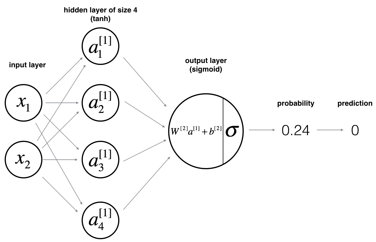
Mathematically:
For one example \(x^{(i)}\):
Given the predictions on all the examples, you can also compute the cost \(J\) as follows:
Reminder: The general methodology to build a Neural Network is to:
1. Define the neural network structure ( # of input units,  # of hidden units, etc).
2. Initialize the model's parameters
3. Loop:
    - Implement forward propagation
    - Compute loss
    - Implement backward propagation to get the gradients
    - Update parameters (gradient descent)
You often build helper functions to compute steps 1-3 and then merge them into one function we call nn_model(). Once you've built nn_model() and learnt the right parameters, you can make predictions on new data.
4.1 - Defining the neural network structure
# GRADED FUNCTION: layer_sizes

def layer_sizes(X, Y):
    """
    Arguments:
    X -- input dataset of shape (input size, number of examples)
    Y -- labels of shape (output size, number of examples)

    Returns:
    n_x -- the size of the input layer
    n_h -- the size of the hidden layer
    n_y -- the size of the output layer
    """
    ### START CODE HERE ### (≈ 3 lines of code)
    n_x = X.shape[0] # size of input layer
    n_h = 4
    n_y = Y.shape[0] # size of output layer
    ### END CODE HERE ###
    return (n_x, n_h, n_y)
4.2 - Initialize the model's parameters
# GRADED FUNCTION: initialize_parameters

def initialize_parameters(n_x, n_h, n_y):
    """
    Argument:
    n_x -- size of the input layer
    n_h -- size of the hidden layer
    n_y -- size of the output layer

    Returns:
    params -- python dictionary containing your parameters:
                    W1 -- weight matrix of shape (n_h, n_x)
                    b1 -- bias vector of shape (n_h, 1)
                    W2 -- weight matrix of shape (n_y, n_h)
                    b2 -- bias vector of shape (n_y, 1)
    """

    np.random.seed(2) # we set up a seed so that your output matches ours although the initialization is random.

    ### START CODE HERE ### (≈ 4 lines of code)
    W1 = np.random.randn(n_h, n_x) * 0.01
    b1 = np.zeros((n_h, 1))
    W2 = np.random.randn(n_y, n_h) * 0.01
    b2 = np.zeros((n_y, 1))
    ### END CODE HERE ###

    assert (W1.shape == (n_h, n_x))
    assert (b1.shape == (n_h, 1))
    assert (W2.shape == (n_y, n_h))
    assert (b2.shape == (n_y, 1))

    parameters = {"W1": W1,
                  "b1": b1,
                  "W2": W2,
                  "b2": b2}

    return parameters
4.3 - The Loop
注意, 若换激活函数,有两个地方需要改:
- forward_propagation()中 A1 = np.tanh(Z1)处;
- backward_propagation()中 dZ1中 1 - np.power(A1, 2) 处.
# GRADED FUNCTION: forward_propagation

def forward_propagation(X, parameters):
    """
    Argument:
    X -- input data of size (n_x, m)
    parameters -- python dictionary containing your parameters (output of initialization function)

    Returns:
    A2 -- The sigmoid output of the second activation
    cache -- a dictionary containing "Z1", "A1", "Z2" and "A2"
    """
    # Retrieve each parameter from the dictionary "parameters"
    ### START CODE HERE ### (≈ 4 lines of code)
    W1 = parameters["W1"]
    b1 = parameters["b1"]
    W2 = parameters["W2"]
    b2 = parameters["b2"]
    ### END CODE HERE ###

    # Implement Forward Propagation to calculate A2 (probabilities)
    ### START CODE HERE ### (≈ 4 lines of code)
    Z1 = np.dot(W1, X) + b1
    A1 = np.tanh(Z1)
    Z2 = np.dot(W2, A1) + b2
    A2 = sigmoid(Z2)
    ### END CODE HERE ###

    assert(A2.shape == (1, X.shape[1]))

    cache = {"Z1": Z1,
             "A1": A1,
             "Z2": Z2,
             "A2": A2}

    return A2, cache
# GRADED FUNCTION: compute_cost

def compute_cost(A2, Y, parameters):
    """
    Computes the cross-entropy cost given in equation (13)

    Arguments:
    A2 -- The sigmoid output of the second activation, of shape (1, number of examples)
    Y -- "true" labels vector of shape (1, number of examples)
    parameters -- python dictionary containing your parameters W1, b1, W2 and b2

    Returns:
    cost -- cross-entropy cost given equation (13)
    """

    m = Y.shape[1] # number of example

    # Compute the cross-entropy cost
    ### START CODE HERE ### (≈ 2 lines of code)
    logprobs = np.multiply(np.log(A2), Y) + np.multiply(np.log(1 - A2), 1 - Y)
    cost = -np.sum(logprobs)/m
    ### END CODE HERE ###

    cost = np.squeeze(cost)     # makes sure cost is the dimension we expect.
                                # E.g., turns [[17]] into 17
    assert(isinstance(cost, float))

    return cost
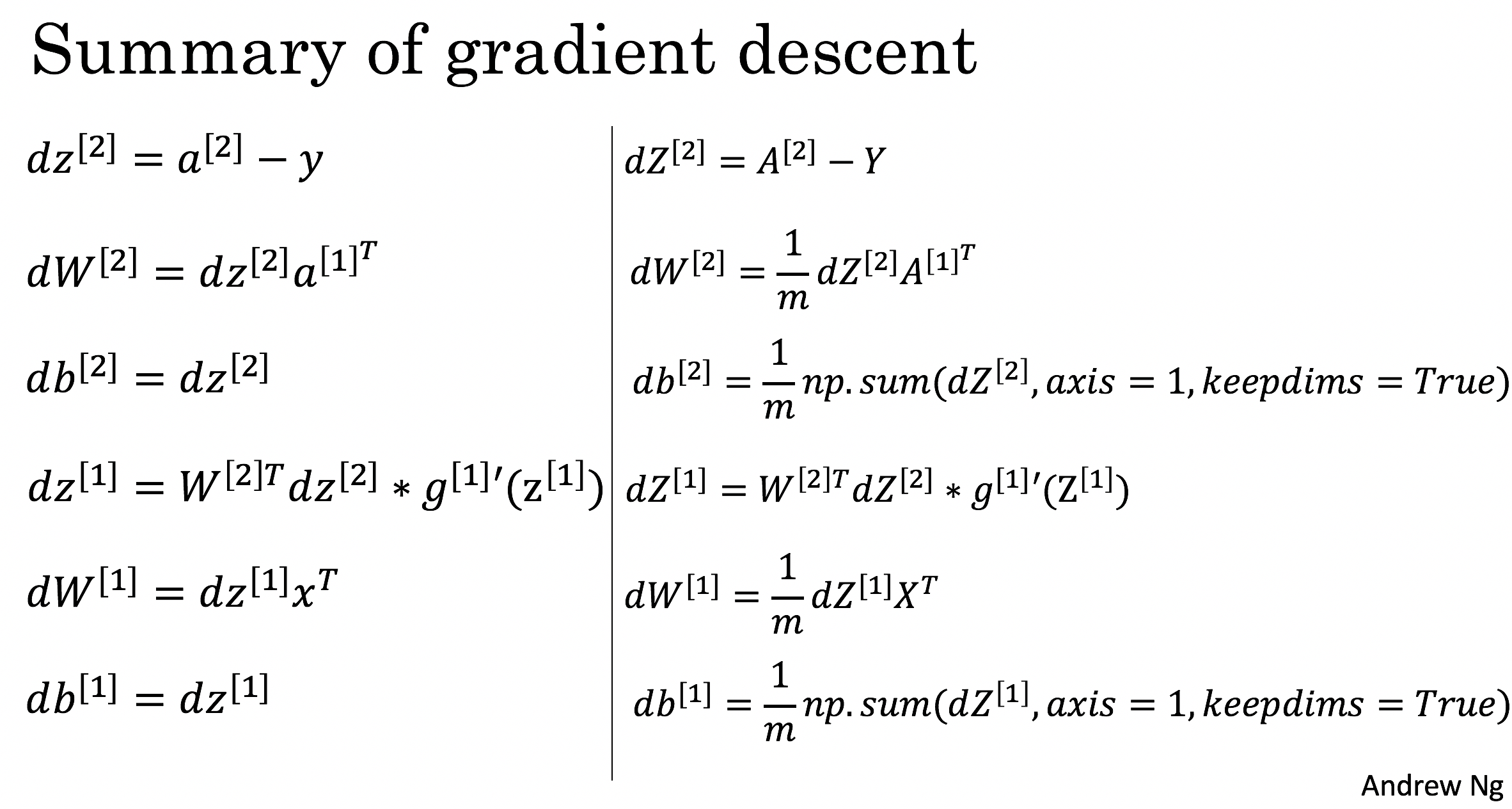
反向传播时用到的公式:
# GRADED FUNCTION: backward_propagation

def backward_propagation(parameters, cache, X, Y):
    """
    Implement the backward propagation using the instructions above.

    Arguments:
    parameters -- python dictionary containing our parameters
    cache -- a dictionary containing "Z1", "A1", "Z2" and "A2".
    X -- input data of shape (2, number of examples)
    Y -- "true" labels vector of shape (1, number of examples)

    Returns:
    grads -- python dictionary containing your gradients with respect to different parameters
    """
    m = X.shape[1]

    # First, retrieve W1 and W2 from the dictionary "parameters".
    ### START CODE HERE ### (≈ 2 lines of code)
    W1 = parameters["W1"]
    W2 = parameters["W2"]
    ### END CODE HERE ###

    # Retrieve also A1 and A2 from dictionary "cache".
    ### START CODE HERE ### (≈ 2 lines of code)
    A1 = cache["A1"]
    A2 = cache["A2"]
    ### END CODE HERE ###

    # Backward propagation: calculate dW1, db1, dW2, db2.
    ### START CODE HERE ### (≈ 6 lines of code, corresponding to 6 equations on slide above)
    dZ2 = A2 - Y
    dW2 = np.dot(dZ2, A1.T)/m
    db2 = np.sum(dZ2, axis=1, keepdims=True)/m

    # tanh的导数 1-A1^2
    # 若换激活函数,有两个地方需要改
    # 1. forward_propagation()中 A1 = np.tanh(Z1)处
    # 2. 就是这里backward_propagation()中 dZ1中 1 - np.power(A1, 2) 处

    dZ1 = np.multiply(np.dot(W2.T, dZ2), 1 - np.power(A1, 2))  # <--
    dW1 = np.dot(dZ1, X.T)/m
    db1 = np.sum(dZ1, axis=1, keepdims=True)/m
    ### END CODE HERE ###

    grads = {"dW1": dW1,
             "db1": db1,
             "dW2": dW2,
             "db2": db2}

    return grads
# GRADED FUNCTION: update_parameters

def update_parameters(parameters, grads, learning_rate = 1.2):
    """
    Updates parameters using the gradient descent update rule given above

    Arguments:
    parameters -- python dictionary containing your parameters
    grads -- python dictionary containing your gradients

    Returns:
    parameters -- python dictionary containing your updated parameters
    """
    # Retrieve each parameter from the dictionary "parameters"
    ### START CODE HERE ### (≈ 4 lines of code)
    W1 = parameters["W1"]
    b1 = parameters["b1"]
    W2 = parameters["W2"]
    b2 = parameters["b2"]
    ### END CODE HERE ###

    # Retrieve each gradient from the dictionary "grads"
    ### START CODE HERE ### (≈ 4 lines of code)
    dW1 = grads["dW1"]
    db1 = grads["db1"]
    dW2 = grads["dW2"]
    db2 = grads["db2"]
    ## END CODE HERE ###

    # Update rule for each parameter
    ### START CODE HERE ### (≈ 4 lines of code)
    W1 -= learning_rate*dW1
    b1 -= learning_rate*db1
    W2 -= learning_rate*dW2
    b2 -= learning_rate*db2
    ### END CODE HERE ###

    parameters = {"W1": W1,
                  "b1": b1,
                  "W2": W2,
                  "b2": b2}

    return parameters
4.4 - Integrate parts 4.1, 4.2 and 4.3 in nn_model()
# GRADED FUNCTION: nn_model

def nn_model(X, Y, n_h, num_iterations = 10000, print_cost=False):
    """
    Arguments:
    X -- dataset of shape (2, number of examples)
    Y -- labels of shape (1, number of examples)
    n_h -- size of the hidden layer
    num_iterations -- Number of iterations in gradient descent loop
    print_cost -- if True, print the cost every 1000 iterations

    Returns:
    parameters -- parameters learnt by the model. They can then be used to predict.
    """

    np.random.seed(3)
    n_x = layer_sizes(X, Y)[0]
    n_y = layer_sizes(X, Y)[2]

    # Initialize parameters, then retrieve W1, b1, W2, b2. Inputs: "n_x, n_h, n_y". Outputs = "W1, b1, W2, b2, parameters".
    ### START CODE HERE ### (≈ 5 lines of code)
    parameters = initialize_parameters(n_x, n_h, n_y)
    W1 = parameters["W1"]
    b1 = parameters["b1"]
    W2 = parameters["W2"]
    b2 = parameters["b2"]
    ### END CODE HERE ###

    # Loop (gradient descent)

    for i in range(0, num_iterations):

        ### START CODE HERE ### (≈ 4 lines of code)
        # Forward propagation. Inputs: "X, parameters". Outputs: "A2, cache".
        A2, cache = forward_propagation(X, parameters)

        # Cost function. Inputs: "A2, Y, parameters". Outputs: "cost".
        cost = compute_cost(A2, Y, parameters)

        # Backpropagation. Inputs: "parameters, cache, X, Y". Outputs: "grads".
        grads = backward_propagation(parameters, cache, X, Y)

        # Gradient descent parameter update. Inputs: "parameters, grads". Outputs: "parameters".
        parameters = update_parameters(parameters, grads)

        ### END CODE HERE ###

        # Print the cost every 1000 iterations
        if print_cost and i % 1000 == 0:
            print ("Cost after iteration %i: %f" %(i, cost))

    return parameters
4.5 Predictions
Reminder: predictions = \(y_{prediction} = \mathbb 1 \text{{activation > 0.5}} = \begin{cases} 1 & \text{if}\ activation > 0.5 \\ 0 & \text{otherwise} \end{cases}\)
As an example, if you would like to set the entries of a matrix X to 0 and 1 based on a threshold you would do: X_new = (X > threshold)
# GRADED FUNCTION: predict

def predict(parameters, X):
    """
    Using the learned parameters, predicts a class for each example in X

    Arguments:
    parameters -- python dictionary containing your parameters
    X -- input data of size (n_x, m)

    Returns
    predictions -- vector of predictions of our model (red: 0 / blue: 1)
    """

    # Computes probabilities using forward propagation, and classifies to 0/1 using 0.5 as the threshold.
    ### START CODE HERE ### (≈ 2 lines of code)
    A2, cache = forward_propagation(X, parameters)
    predictions = (A2[0] > 0.5)  # [ True False  True] 而不是 [1 0 1]
    ### END CODE HERE ###

    return predictions
使用模型
# Build a model with a n_h-dimensional hidden layer
# 模型经训练后,最终得到 parameters = W2, b2, W1, b1
parameters = nn_model(X, Y, n_h = 4, num_iterations = 10000, print_cost=True)

# Plot the decision boundary
# 新数据 x 和训练好的参数 parameters 送入 predict() 后, 经过一个前向, 得到A2,
# 再经threshold得到预测结果.
# Print accuracy
predictions = predict(parameters, X)
print ('Accuracy: %d' % float((np.dot(Y,predictions.T) + np.dot(1-Y,1-predictions.T))/float(Y.size)*100) + '%')
4.6 - Tuning hidden layer size (optional/ungraded exercise)
plt.figure(figsize=(16, 32))
hidden_layer_sizes = [1, 2, 3, 4, 5, 10, 20]
for i, n_h in enumerate(hidden_layer_sizes):
    plt.subplot(5, 2, i+1)
    plt.title('Hidden Layer of size %d' % n_h)
    parameters = nn_model(X, Y, n_h, num_iterations = 5000)
    plot_decision_boundary(lambda x: predict(parameters, x.T), X, Y)
    predictions = predict(parameters, X)
    accuracy = float((np.dot(Y,predictions.T) + np.dot(1-Y,1-predictions.T))/float(Y.size)*100)
    print ("Accuracy for {} hidden units: {} %".format(n_h, accuracy))
最后顺便把作业里的两个动画(表现学习率设置不合适导致发散,反过来收敛)也弄上来:

【推荐】编程新体验,更懂你的AI,立即体验豆包MarsCode编程助手
【推荐】凌霞软件回馈社区,博客园 & 1Panel & Halo 联合会员上线
【推荐】抖音旗下AI助手豆包,你的智能百科全书,全免费不限次数
【推荐】轻量又高性能的 SSH 工具 IShell:AI 加持,快人一步