Deep Learning Specialization 笔记

1. numpy中的几种矩阵相乘:

# x1: axn, x2:nxb

np.dot(x1, x2): axn * nxb

np.outer(x1, x2): nx1*1xn    # 实质为: np.ravel(x1)*np.ravel(x2)

np.multiply(x1, x2): [[x1[0][0]*x2[0][0], x1[0][1]*x2[0][1], ...]

2. Bugs' hometown

Many software bugs in deep learning come from having matrix/vector dimensions that don't fit. If you can keep your matrix/vector dimensions straight you will go a long way toward eliminating many bugs.

3. Common steps for pre-processing a new dataset are:

- Figure out the dimensions and shapes of the problem (m_train, m_test, num_px, ...) - Reshape the datasets such that each example is now a vector of size (num_px \* num_px \* 3, 1) - "Standardize" the data

4. Unstructured data:

Unstructured data is a generic label for describing data that is not contained in a database or some other type of data structure . Unstructured data can be textual or non-textual. Textual unstructured data is generated in media like email messages, PowerPoint presentations, Word documents, collaboration software and instant messages. Non-textual unstructured data is generated in media like JPEG images, MP3 audio files and Flash video files

5. Chapter of Activation Function:

• Choice of activation function:

  1. If output is either 0 or 1 -- sigmoid for the output layer and the other units on ReLU.
  2. Except for the output layer, tanh does better than sigmoid.
  3. ReLU ---level up--> leaky ReLU.

• Why are ReLU and leaky ReLU often superior to sigmoid and tanh?

  -- The derivatives of the former ones is much bigger than 0, so the learning would be much faster.

• A linear hidden layer is more or less useless, yet the activation function is a exception.

6. Regularization:

Initially, \(J(w, b) = \frac{1}{m} * \sum_{i=1}^{m}{L({\hat{Y}^(i), y^{(i)}}) + \frac{\lambda}{2*m}||w||_2^2}\)

1. L2 regularization: \(\frac{\lambda}{2*m}\sum_{j=1}^{n_x}||w_j||^2 = \frac{\lambda}{2*m}||w||_2\)

   One aspect that tanh is better thatn sigmoid(in terms of regularization) -- When x is very close to 0, the derivative of tanh(x) is almost linear, while that of the sigmoid(x) is alomst 0.

2. Dropout:

     Method: Make certain values of weights be zeros randomly, just like -- W= np.multiply(W, C), where C is a 0-1 array.

     Matters need attention: Don't use dropout in test procedure -- Time costly, result randomly.

     Work principle:

       Intuition: Can't rely on any one feature, so have to spread out weights(shrinking weights).

       Besides, you can set different rates of "Dropout", like lower ones on more complex layer, which are called "key prop".

3. Data augmentation:

     Do some operation on your data images, such as flipping, rotation, zooming, etc, without changing their labels, in order to prevent from over-fitting on some aspects, such as the direction of faces, the size of cats.

4. Early stopping.

7. Solution to "gradient vanishing or exploding":

     Set W^L = np.random.randn(shape) * np.sqrt(\(\frac{2}{n^{[L-1]}}\)) if activation_function == "ReLU"
       else: np.random.randn(shape) * np.sqrt(\(\frac{1}{n^{[L-1]}}\)) or np.sqrt(\(\sqrt{\frac{2}{n^{[L-1]}+n^{[L]}}}\))(Xavier initialization)

8. Gradient Checking:

1. for i in range(len(\(\theta\))):

   to check if (d\(\theta_{approx}[i] = \frac{J(\theta_1, \theta_2, ..., \theta_i+\epsilon, ...) - J(\theta_1, \theta_2, ..., \theta_i-\epsilon, ...)}{2\epsilon}\)) ?= \(d\theta[i] = \frac{\partial{J}}{\partial{\theta_i}}\)

            <==> \(d\theta_{approx} ?= d\theta\)

            <==> \(\frac{||d\theta_{approx} - d\theta||_2}{||d\theta_{approx}||_2+||d\theta||_2}\) in an accent range: \(10^{-7}\) is great, and \(10^{-3}\) is wrong.

2. Tips:

   • Only to debug, instead of training.
   • If algorithm fails grad check, look at components(\(db^{[L]}, dw^{[L]}\)) to try to identify bug.
   • Remember regularization.
   • Doesn't work together with dropout.
   • Run at random initialization; perhaps again after some training.

9. Exponentially weighted averages:

  Definition: let \(V_{t} = {\beta}V_{t-1} + (1 - \beta)\theta_t\) (_V_s are the averages, and the _\(\theta\)_s are the initial discrete data).

and \(V_{t} = \frac{V_{t}}{1 - {\beta}^t}\) (To correct initial bias).

  Usage: when it comes to this situation: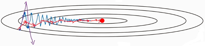
Since the average of the distance vertical movement is almost zeros, you can use EWA to average it, prevent it from divergence.
  On iteration t:
    Compute dW on the current mini-batch
    \(v_{dW} = {\beta}v_{dW} + (1 - \beta)dW\)
    \(v_{db} = {\beta}v_{db} + (1 - \beta)db\)
    \(W = W - {\alpha}v_{dW}, b = b - {\alpha}v_{db}\)
    Hyperparameters: \(\alpha\), \({\beta}(=0.9)\)