吴恩达 — 神经网络与深度学习 — L1W2编程作业


 第二周编程作业


In [8]:
import numpy as np
import matplotlib.pyplot as plt
import h5py
In [69]:
def load_dataset():
    # 读入训练数据    
    train_datasets = h5py.File('./datasets/train_catvnoncat.h5')
    train_x = np.array(train_datasets['train_set_x'][:])
    train_y = np.array(train_datasets['train_set_y'][:])
    # 读入测试数据
    test_datasets = h5py.File('./datasets/test_catvnoncat.h5')
    test_x = np.array(test_datasets['test_set_x'][:])
    test_y = np.array(test_datasets['test_set_y'][:])
    # 读入类别
    classes = np.array(test_datasets['list_classes'][:])
    # 改变标签的维度,避免rank1数据结构
    print(train_y.shape)
    train_y = train_y.reshape((1, train_y.shape[0]))
    test_y = test_y.reshape((1, test_y.shape[0]))
    print(train_y.shape)
    
    return train_x, train_y, test_x, test_y, classes
In [70]:
# 读取数据
train_x, train_y, test_x, test_y, classes = load_dataset()
 
(209,)
(1, 209)
In [99]:
# index属于[0, 209)
index = int(np.random.rand()*train_x.shape[0])
print("index = {0:d}".format(index))
plt.title(classes[train_y[0][index]])
plt.imshow(train_x[index])
 
index = 117
Out[99]:
<matplotlib.image.AxesImage at 0x2a19b066748>
 
In [101]:
# np.squeeze(train_y[:,index])是为了压缩维度,未压缩前为[1],压缩后为1
print("y=" + str(train_y[:,index]) + ", it's a " + classes[np.squeeze(train_y[:,index])].decode("utf-8") + "' picture")
 
y=[1], it's a cat' picture
 

m_train: 训练集里面的图片数量

m_test: 测试集里面的图片数量

num_px: 训练,测试集里面图形的高度和宽度(64*64)

train_x维度: (m_train, num_px, num_px, 3)

test_x维度: (m_test, num_px, num_px, 3)

train_y维度: (1, m_train)

test_y维度: (1, m_test)

In [109]:
m_train = train_x.shape[0]
m_test = test_y.shape[0]
num_px = train_x.shape[1]

print('训练集的数量: m_train={:d}'.format(m_train))
print('测试集的数量: m_test={:d}'.format(m_test))
print('图片的像素点宽高: num_px={:d}'.format(num_px))
print('每张图片大小({0:d},{1:d},{2:d})'.format(num_px, num_px, 3))
print('训练数据图片维度: train_x={:}'.format(train_x.shape))
print('训练数据标签维度: train_y={:}'.format(train_y.shape))
print('测试数据图片维度: train_x={:}'.format(test_x.shape))
print('测试数据标签维度: train_y={:}'.format(test_y.shape))
 
训练集的数量: m_train=209
测试集的数量: m_test=1
图片的像素点宽高: num_px=64
每张图片大小(64,64,3)
训练数据图片维度: train_x=(209, 64, 64, 3)
训练数据标签维度: train_y=(1, 209)
测试数据图片维度: train_x=(50, 64, 64, 3)
测试数据标签维度: train_y=(1, 50)
 

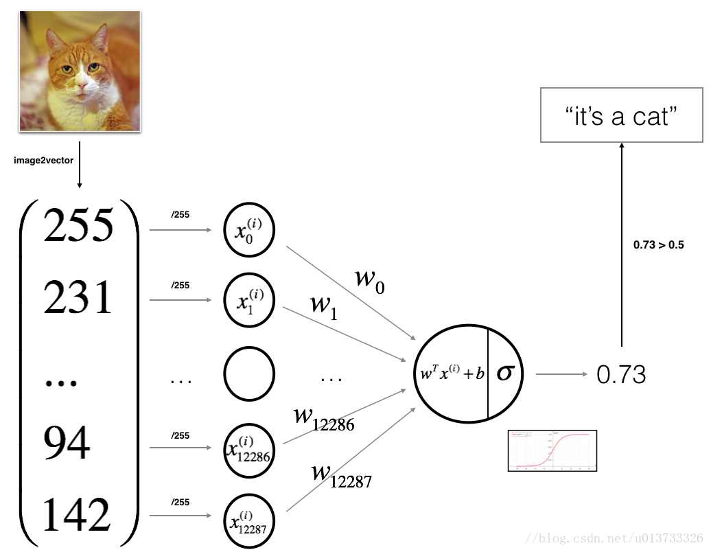
为了方便起见,我们将维度(64,64,3)的numpy数组转变为(64643,1)的数组 乘3的原因是因为每张图片由64*64的像素点构成,每个像素点由RGB三通道构成 所以要乘3。之后训练集和测试集得到了两个numpy数组,每列代表一个平坦的图形 应该由m_train列,m_test列

In [113]:
# .T表示矩阵的转置
# reshape中的-1表示让计算机计算这个维度,但只可以有一个-1,比如(209,64,64,3)reshape为(209,-1),计算机会计算-1为64*64*3=12288
# 加上转置后,每一列相当于一个平坦的图像
train_x_flat = train_x.reshape(train_x.shape[0], -1).T
test_x_flat = test_x.reshape(test_x.shape[0], -1).T
In [115]:
print('训练数据降维后的维度: train_x={:}'.format(train_x_flat.shape))
print('训练数据标签维度: train_y={:}'.format(train_y.shape))
print('测试数据降维后的维度: train_x={:}'.format(test_x_flat.shape))
print('测试数据标签维度: train_y={:}'.format(test_y.shape))
 
训练数据降维后的维度: train_x=(12288, 209)
训练数据标签维度: train_y=(1, 209)
测试数据降维后的维度: train_x=(12288, 50)
测试数据标签维度: train_y=(1, 50)
 

为了表示彩色图像,必须为每个像素指定红色,绿色和蓝色通道(RGB),因此像素值实际上是从0到255范围内的三个数字的向量。机器学习中一个常见的预处理步骤是对数据集进行居中和标准化,这意味着可以减去每个示例中整个numpy数组的平均值,然后将每个示例除以整个numpy数组的标准偏差。但对于图片数据集,它更简单,更方便,几乎可以将数据集的每一行除以255(像素通道的最大值),因为在RGB中不存在比255大的数据,所以我们可以放心的除以255,让标准化的数据位于[0,1]之间,现在标准化我们的数据集:

In [117]:
# 数据标准化
train_x = train_x_flat/255
test_x = test_x_flat/255
 

jupyter


jupyter


建立神经网络步骤

1.定义好模型结构,如输入特征数量,权值数组,偏置

2.初始化模型参数

3.循环

3.1 计算当前损失(forward propagation)

3.2 计算当前梯度(backward propagation)

3.3 更新参数(gradient descent)

activation function:sigmoid()函数

要使用sigmoid计算预测值

In [126]:
def sigmoid(z):
    '''
    参数:
        z - 任意numpy数组
    返回:
        return - sigmoid(z)
    '''
    return 1/(1+np.exp(-z))
In [133]:
# 测试sigmoid函数
# 可以看出值越大,或者越小,梯度越小
print('sigmoid(0) = {:.3}, g\'(0) = {:.3}'.format(sigmoid(0), sigmoid(0)*(1-sigmoid(0))))
print('sigmoid(10) = {:.3}, g\'(5) = {:.3}'.format(sigmoid(5), sigmoid(5)*(1-sigmoid(5))))
print('sigmoid(-10) = {:.3}, g\'(-5) = {:.3}'.format(sigmoid(-5), sigmoid(-5)*(1-sigmoid(-5))))
 
sigmoid(0) = 0.5, g'(0) = 0.25
sigmoid(10) = 0.993, g'(5) = 0.00665
sigmoid(-10) = 0.00669, g'(-5) = 0.00665
 

sigmoid函数定义好了,接下来定义初始化权值参数w和偏置b

In [176]:
def initialize_with_zero(dim):
    '''
    此函数为w创建一个维度为(dim,1)的0向量,b初始化为0
    参数:
        dim - 表示w的维度
    返回
        w - 维度为(dim, 1)的列向量
        b - 偏置,值为0
    '''
    w = np.zeros((dim, 1))
    b = 0
    # 用断言来判断数据是否符合条件    
    assert(w.shape == (dim, 1)) #判断w维度是否是(dim,1)
    assert(isinstance(b, float) or isinstance(b, int))#判断b是否是浮点型或者整形
    return w, b
 

初始化参数的函数已经定义好了

现在我们定义'前向'和'反向传播',来学习参数

In [205]:
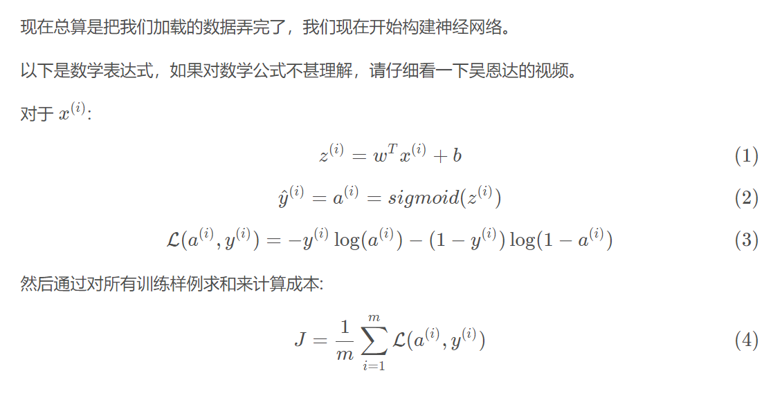
def propagate(w, b, X, Y):
    '''
    实现前向和反向传播计算成本函数和梯度
    参数:
        w - 权值,一个维度为(num_px*num_px*3,1)的数据
        b - 偏置,一个标量
        X - 训练数据,维度为(num_px*num_px*3, m_train)
        Y - 训练数据标签,维度为(1, m_train)
    返回:
        cost - 逻辑回归的负对数最大似然成本
        dw - 权值数组w的损失梯度,与w的shape一致
        db - b的损失梯度,与b的shape一致
    '''
    epsilon = 1e-5
    m = X.shape[1]
    # 正向传播
    # w.T.shape=(1, num_px*num_px*3), X.shape=(num_px*num_px*3, m)
    Z = np.dot(w.T, X)+b #shape=(1, m)
    A = sigmoid(Z)
    cost = (-1/m)*np.sum(Y*np.log(A+epsilon)+(1-Y)*np.log(1-A+epsilon))
    
    #反向传播
    dz = A-Y #shape(1,m)
    dw = (1/m)*np.dot(X, dz.T)
    db = (1/m)*np.sum(dz)
    
    #使用断言确保数据正确
    assert(dw.shape==w.shape)
    assert(db.dtype==float)
    cost = np.squeeze(cost)
    assert(cost.shape==())
    
    #创建一个字典把dw,db存起来
    grads = {
        'dw':dw,
        'db':db
    }
    return (grads, cost)
In [156]:
#测试一下propagate
print("------propagate------")
# 初始化一些参数
w, b, X, Y = np.array([[1],[2]]), 1.2, np.array([[1,0],[2,0.5]]), np.array([[1, 0]])
grads, cost = propagate(w, b, X, Y)
print("dw = {:}".format(grads['dw']))
print("db = {:}".format(grads['db']))
print("cost = {:}".format(cost))
 
------propagate------
dw = [[-0.00101266]
 [ 0.22303706]]
db = 0.44911209524563245
cost = 1.1535553469462667
 

目标是通过最小化成本函数J来学习w和b

α为学习率

更新规则为:

w = w-αdw

b = b-αdb

In [242]:
def optimize(w, b, X, Y, num_iterations, learning_rate, print_cost):
    '''
    此函数使用梯度下降法最小化成本函数J优化参数w和b
    参数:
        w - 权值参数,维度为(num_px*num_px*3, 1)的数组
        b - 偏置,一个标量
        X - 训练数据,维度为(num_px*num_px*3, m_train)的数组
        Y - 训练数据标签,维度为(1, m_train)的数组
        num_iterations - 优化迭代的次数
        learning_rate - 学习率
        print_cost - 每一百步打印一次损失值
    返回:
        params - 包含权值w和偏置b的字典
        grads - 包含当前成本函数对权值w和b的梯度字典
        costs - 优化迭代期间保存的成本损失
    提示:
    我们需要写下两个步骤来进行迭代优化
        1,计算当前参数的成本和梯度,使用propagate()函数
        2,使用梯度下降法更新w,b
    '''
    costs = []
    for i in range(num_iterations):
        grads, cost = propagate(w, b, X, Y)
        dw = grads['dw']
        db = grads['db']
        
        #梯度下降法更新参数
        w = w-learning_rate*dw
        b = b-learning_rate*db
        
        if(i%100==0):
            # 记录成本
            costs.append(cost)
            #print(costs)
        if(print_cost) and (i%100==0):
            print("迭代次数{:d}, cost={:}".format(i, cost))
    params = {
        'w':w,
        'b':b,
    }
    grads = {
        'dw':dw,
        'db':db,
    }
    return (params, grads, costs)
In [163]:
#测试一下optimize
print("------optimize------")
# 初始化一些参数
w, b, X, Y = np.array([[1],[2]]), 1.2, np.array([[1,0],[2,0.5]]), np.array([[1, 0]])
params, grads, costs = optimize(w, b, X, Y, 10000, 0.01, True)
print("w = {:}".format(params['w']))
print("b = {:}".format(params['b']))
print("dw = {:}".format(grads['dw']))
print("db = {:}".format(grads['db']))
print("costs = {:}".format(costs))
 
------optimize------
迭代次数0, cost=1.1535553469462667
迭代次数100, cost=0.918666053293677
迭代次数200, cost=0.7230081821112836
迭代次数300, cost=0.5716021904653603
迭代次数400, cost=0.46257241533117516
迭代次数500, cost=0.38825180308883256
迭代次数600, cost=0.3386564650889955
迭代次数700, cost=0.30477307040281393
迭代次数800, cost=0.280160561294915
迭代次数900, cost=0.2609172176169882
迭代次数1000, cost=0.24491471733497527
迭代次数1100, cost=0.2310430562944525
迭代次数1200, cost=0.21871540239514628
迭代次数1300, cost=0.2076004417155667
迭代次数1400, cost=0.19749147074735043
迭代次数1500, cost=0.1882451724314827
迭代次数1600, cost=0.17975314721079405
迭代次数1700, cost=0.1719283161376686
迭代次数1800, cost=0.1646980450006676
迭代次数1900, cost=0.15800036338549817
迭代次数2000, cost=0.15178166816416494
迭代次数2100, cost=0.14599518514380458
迭代次数2200, cost=0.14059985121125318
迭代次数2300, cost=0.13555945248895263
迭代次数2400, cost=0.13084193311054632
迭代次数2500, cost=0.1264188266587977
迭代次数2600, cost=0.12226478090496268
迭代次数2700, cost=0.11835715631935917
迭代次数2800, cost=0.11467568441832025
迭代次数2900, cost=0.11120217546102526
迭代次数3000, cost=0.1079202673026805
迭代次数3100, cost=0.10481520883736711
迭代次数3200, cost=0.10187367267751883
迭代次数3300, cost=0.09908359265575156
迭代次数3400, cost=0.09643402247936361
迭代次数3500, cost=0.09391501246862093
迭代次数3600, cost=0.09151750180047369
迭代次数3700, cost=0.08923322408320693
迭代次数3800, cost=0.08705462442209087
迭代次数3900, cost=0.08497478641457781
迭代次数4000, cost=0.0829873677462934
迭代次数4100, cost=0.08108654325418187
迭代次数4200, cost=0.07926695448722473
迭代次数4300, cost=0.07752366493350055
迭代次数4400, cost=0.07585212019930794
迭代次数4500, cost=0.07424811252518282
迭代次数4600, cost=0.07270774910784027
迭代次数4700, cost=0.07122742376874819
迭代次数4800, cost=0.06980379157121322
迭代次数4900, cost=0.06843374604016628
迭代次数5000, cost=0.06711439868366753
迭代次数5100, cost=0.06584306055365267
迭代次数5200, cost=0.06461722561657429
迭代次数5300, cost=0.06343455573316861
迭代次数5400, cost=0.06229286707126022
迭代次数5500, cost=0.06119011779689494
迭代次数5600, cost=0.060124396907623695
迭代次数5700, cost=0.05909391408787547
迭代次数5800, cost=0.058096990480374436
迭代次数5900, cost=0.05713205027979186
迭代次数6000, cost=0.05619761306550955
迭代次数6100, cost=0.05529228679971891
迭代次数6200, cost=0.05441476142528336
迭代次数6300, cost=0.05356380300498792
迭代次数6400, cost=0.05273824835013177
迭代次数6500, cost=0.05193700009199803
迭代次数6600, cost=0.05115902215465493
迭代次数6700, cost=0.050403335591893056
迭代次数6800, cost=0.049669014754948185
迭代次数6900, cost=0.0489551837610739
迭代次数7000, cost=0.04826101323605007
迭代次数7100, cost=0.04758571730640648
迭代次数7200, cost=0.046928550819535404
迭代次数7300, cost=0.04628880677199623
迭代次数7400, cost=0.04566581392822354
迭代次数7500, cost=0.04505893461354926
迭代次数7600, cost=0.04446756266696828
迭代次数7700, cost=0.04389112154044697
迭代次数7800, cost=0.04332906253278744
迭代次数7900, cost=0.04278086314716668
迭代次数8000, cost=0.04224602556244834
迭代次数8100, cost=0.041724075209260525
迭代次数8200, cost=0.0412145594426255
迭代次数8300, cost=0.0407170463036547
迭代次数8400, cost=0.04023112336347016
迭代次数8500, cost=0.039756396643105145
迭代次数8600, cost=0.039292489603666395
迭代次数8700, cost=0.038839042201525696
迭代次数8800, cost=0.038395710003745614
迭代次数8900, cost=0.03796216335934046
迭代次数9000, cost=0.037538086622333613
迭代次数9100, cost=0.0371231774229025
迭代次数9200, cost=0.03671714598320118
迭代次数9300, cost=0.03631971447471724
迭代次数9400, cost=0.035930616414276556
迭代次数9500, cost=0.03554959609602615
迭代次数9600, cost=0.0351764080569406
迭代次数9700, cost=0.034810816573579165
迭代次数9800, cost=0.034452595187998876
迭代次数9900, cost=0.03410152626088485
w = [[3.16844931]
 [2.51947271]]
b = -4.266402490851132
dw = [[-0.00953026]
 [-0.00727794]]
db = 0.014034888793961777
costs = [1.1535553469462667, 0.918666053293677, 0.7230081821112836, 0.5716021904653603, 0.46257241533117516, 0.38825180308883256, 0.3386564650889955, 0.30477307040281393, 0.280160561294915, 0.2609172176169882, 0.24491471733497527, 0.2310430562944525, 0.21871540239514628, 0.2076004417155667, 0.19749147074735043, 0.1882451724314827, 0.17975314721079405, 0.1719283161376686, 0.1646980450006676, 0.15800036338549817, 0.15178166816416494, 0.14599518514380458, 0.14059985121125318, 0.13555945248895263, 0.13084193311054632, 0.1264188266587977, 0.12226478090496268, 0.11835715631935917, 0.11467568441832025, 0.11120217546102526, 0.1079202673026805, 0.10481520883736711, 0.10187367267751883, 0.09908359265575156, 0.09643402247936361, 0.09391501246862093, 0.09151750180047369, 0.08923322408320693, 0.08705462442209087, 0.08497478641457781, 0.0829873677462934, 0.08108654325418187, 0.07926695448722473, 0.07752366493350055, 0.07585212019930794, 0.07424811252518282, 0.07270774910784027, 0.07122742376874819, 0.06980379157121322, 0.06843374604016628, 0.06711439868366753, 0.06584306055365267, 0.06461722561657429, 0.06343455573316861, 0.06229286707126022, 0.06119011779689494, 0.060124396907623695, 0.05909391408787547, 0.058096990480374436, 0.05713205027979186, 0.05619761306550955, 0.05529228679971891, 0.05441476142528336, 0.05356380300498792, 0.05273824835013177, 0.05193700009199803, 0.05115902215465493, 0.050403335591893056, 0.049669014754948185, 0.0489551837610739, 0.04826101323605007, 0.04758571730640648, 0.046928550819535404, 0.04628880677199623, 0.04566581392822354, 0.04505893461354926, 0.04446756266696828, 0.04389112154044697, 0.04332906253278744, 0.04278086314716668, 0.04224602556244834, 0.041724075209260525, 0.0412145594426255, 0.0407170463036547, 0.04023112336347016, 0.039756396643105145, 0.039292489603666395, 0.038839042201525696, 0.038395710003745614, 0.03796216335934046, 0.037538086622333613, 0.0371231774229025, 0.03671714598320118, 0.03631971447471724, 0.035930616414276556, 0.03554959609602615, 0.0351764080569406, 0.034810816573579165, 0.034452595187998876, 0.03410152626088485]
 

optimize()函数会计算得到优化后的参数w,b,我们可以使用w,b来预测数据集的标签

现在我们编写optimize()函数只要包括两个步骤

1,A = y hat = sigmoid(w.T+b)
2,如果A<=0,A赋值为0,如果A>0.5,A赋值为1

然后将预测值存入:Y_prediction

In [167]:
def predict(w, b, X):
    '''
    此函数使用参数w,b来预测X的标签为0还是1
    参数:
        w - 权值参数,维度为(num_px*num_px*3, 1)的数组
        b - 偏置,一个标量
        X - 预测的样本数据,维度为(num_px*num_px*3, m),m表示样本数量
    返回:
        Y_prediction - X的预测标签,维度为(1, m)
    '''
    m = X.shape[1]
    Y_prediction = np.zeros((1,m))
    w = w.reshape((X.shape[0],1))
    
    # 计算每张图片是cat的概率
    A = np.dot(w.T, X)+b
    for i in range(A.shape[1]):
        # 计算出X对应的标签
        Y_prediction[0, i] = 1 if A[0,i]>0.5 else 0
    # 
    assert(Y_prediction.shape == (1,m))
    return Y_prediction
In [180]:
#测试一下optimize
print("------optimize------")
# 初始化一些参数
w, b, X, Y = np.array([[1],[2]]), 1.2, np.array([[1,0],[2,0.5]]), np.array([[1, 0]])
params, grads, costs = optimize(w, b, X, Y, 10000, 0.01, True)
Y_prediction = predict(params['w'], params['b'], X)
print('predict = {:}'.format(Y_prediction))
 
------optimize------
迭代次数0, cost=1.1535553469462667
迭代次数100, cost=0.918666053293677
迭代次数200, cost=0.7230081821112836
迭代次数300, cost=0.5716021904653603
迭代次数400, cost=0.46257241533117516
迭代次数500, cost=0.38825180308883256
迭代次数600, cost=0.3386564650889955
迭代次数700, cost=0.30477307040281393
迭代次数800, cost=0.280160561294915
迭代次数900, cost=0.2609172176169882
迭代次数1000, cost=0.24491471733497527
迭代次数1100, cost=0.2310430562944525
迭代次数1200, cost=0.21871540239514628
迭代次数1300, cost=0.2076004417155667
迭代次数1400, cost=0.19749147074735043
迭代次数1500, cost=0.1882451724314827
迭代次数1600, cost=0.17975314721079405
迭代次数1700, cost=0.1719283161376686
迭代次数1800, cost=0.1646980450006676
迭代次数1900, cost=0.15800036338549817
迭代次数2000, cost=0.15178166816416494
迭代次数2100, cost=0.14599518514380458
迭代次数2200, cost=0.14059985121125318
迭代次数2300, cost=0.13555945248895263
迭代次数2400, cost=0.13084193311054632
迭代次数2500, cost=0.1264188266587977
迭代次数2600, cost=0.12226478090496268
迭代次数2700, cost=0.11835715631935917
迭代次数2800, cost=0.11467568441832025
迭代次数2900, cost=0.11120217546102526
迭代次数3000, cost=0.1079202673026805
迭代次数3100, cost=0.10481520883736711
迭代次数3200, cost=0.10187367267751883
迭代次数3300, cost=0.09908359265575156
迭代次数3400, cost=0.09643402247936361
迭代次数3500, cost=0.09391501246862093
迭代次数3600, cost=0.09151750180047369
迭代次数3700, cost=0.08923322408320693
迭代次数3800, cost=0.08705462442209087
迭代次数3900, cost=0.08497478641457781
迭代次数4000, cost=0.0829873677462934
迭代次数4100, cost=0.08108654325418187
迭代次数4200, cost=0.07926695448722473
迭代次数4300, cost=0.07752366493350055
迭代次数4400, cost=0.07585212019930794
迭代次数4500, cost=0.07424811252518282
迭代次数4600, cost=0.07270774910784027
迭代次数4700, cost=0.07122742376874819
迭代次数4800, cost=0.06980379157121322
迭代次数4900, cost=0.06843374604016628
迭代次数5000, cost=0.06711439868366753
迭代次数5100, cost=0.06584306055365267
迭代次数5200, cost=0.06461722561657429
迭代次数5300, cost=0.06343455573316861
迭代次数5400, cost=0.06229286707126022
迭代次数5500, cost=0.06119011779689494
迭代次数5600, cost=0.060124396907623695
迭代次数5700, cost=0.05909391408787547
迭代次数5800, cost=0.058096990480374436
迭代次数5900, cost=0.05713205027979186
迭代次数6000, cost=0.05619761306550955
迭代次数6100, cost=0.05529228679971891
迭代次数6200, cost=0.05441476142528336
迭代次数6300, cost=0.05356380300498792
迭代次数6400, cost=0.05273824835013177
迭代次数6500, cost=0.05193700009199803
迭代次数6600, cost=0.05115902215465493
迭代次数6700, cost=0.050403335591893056
迭代次数6800, cost=0.049669014754948185
迭代次数6900, cost=0.0489551837610739
迭代次数7000, cost=0.04826101323605007
迭代次数7100, cost=0.04758571730640648
迭代次数7200, cost=0.046928550819535404
迭代次数7300, cost=0.04628880677199623
迭代次数7400, cost=0.04566581392822354
迭代次数7500, cost=0.04505893461354926
迭代次数7600, cost=0.04446756266696828
迭代次数7700, cost=0.04389112154044697
迭代次数7800, cost=0.04332906253278744
迭代次数7900, cost=0.04278086314716668
迭代次数8000, cost=0.04224602556244834
迭代次数8100, cost=0.041724075209260525
迭代次数8200, cost=0.0412145594426255
迭代次数8300, cost=0.0407170463036547
迭代次数8400, cost=0.04023112336347016
迭代次数8500, cost=0.039756396643105145
迭代次数8600, cost=0.039292489603666395
迭代次数8700, cost=0.038839042201525696
迭代次数8800, cost=0.038395710003745614
迭代次数8900, cost=0.03796216335934046
迭代次数9000, cost=0.037538086622333613
迭代次数9100, cost=0.0371231774229025
迭代次数9200, cost=0.03671714598320118
迭代次数9300, cost=0.03631971447471724
迭代次数9400, cost=0.035930616414276556
迭代次数9500, cost=0.03554959609602615
迭代次数9600, cost=0.0351764080569406
迭代次数9700, cost=0.034810816573579165
迭代次数9800, cost=0.034452595187998876
迭代次数9900, cost=0.03410152626088485
predict = [[1. 0.]]
 

把所有函数整合到一个model函数里面完成

In [258]:
def model(X_train, Y_train, X_test, Y_test, num_iterations=2000, learning_rate=0.01, print_cost=False):
    '''
    此函数通过调用前面定义的函数完成logistic regession模型构建
    参数:
        X_train - 训练数据,维度为[num_px*num_px*3, m_train]的数组
        Y_train - 训练数据的标签,维度为[1, m_train]的数组
        Y_train - 测试数据,维度为[num_px*num_px*3, m_test]的数组
        Y_test - 测试数据的标签,维度为[1, m_test]的数组
        num_iterations - 优化迭代的轮数,默认值为2000
        learning_rat - 学习率,默认值为0.1
        print_cost - 每一百轮输出成本损失
    返回
        d - 包含有关模型信息的字典
    '''
    # 初始化权值w和偏置
    w, b = initialize_with_zero(X_train.shape[0])
    
    # 使用梯度下降法最下化成本损失值,优化得到w,b
    params, grads, costs = optimize(w, b, X_train, Y_train, num_iterations, learning_rate, print_cost)
    
    # 取出优化得到的w,b
    w = params['w']
    b = params['b']
    
    # 使用predict()函数预测训练数据和测试数据的标签
    Y_prediction_train = predict(w, b, X_train)
    Y_prediction_test = predict(w, b, X_test)
    
    # 计算准确率
    acc_train = np.sum(Y_prediction_train==Y_train,dtype=np.float64)/Y_train.shape[1]
    acc_test = np.sum(Y_prediction_test==Y_test)/Y_test.shape[1]
    # 打印准确率
    print("训练集准确率为:{:.3}".format(acc_train))
    print("测试集准确率为:{:.3}".format(acc_test))
    d = {
        'w':w,
        'b':b,
        'costs':costs,
        'Y_prediction_train':Y_prediction_train,
        'Y_prediction_test':Y_prediction_test,
        'learning_rate':learning_rate,
        'num_iterations':num_iterations,
    }
    return d
In [256]:
print("------测试model------")
# 这里使用真实数据
d = model(train_x, train_y, test_x, test_y,print_cost=True, learning_rate=0.005, num_iterations=2000)
 
------测试model------
迭代次数0, cost=0.6931271807599427
迭代次数100, cost=0.5844891556710067
迭代次数200, cost=0.46693218875670767
迭代次数300, cost=0.3759917224139368
迭代次数400, cost=0.331448761179504
迭代次数500, cost=0.30325900292045477
迭代次数600, cost=0.27986589707982307
迭代次数700, cost=0.26002875904551354
迭代次数800, cost=0.2429275708800498
迭代次数900, cost=0.22799133583982367
迭代次数1000, cost=0.2148068245330989
迭代次数1100, cost=0.2030656746911994
迭代次数1200, cost=0.19253191458997668
迭代次数1300, cost=0.18302111195618995
迭代次数1400, cost=0.17438649072215992
迭代次数1500, cost=0.16650940359187233
迭代次数1600, cost=0.15929262457127985
迭代次数1700, cost=0.1526555216496732
迭代次数1800, cost=0.14653051472565828
迭代次数1900, cost=0.14086043119707853
训练集准确率为:0.981
测试集准确率为:0.7
In [251]:
# 绘制图
costs = np.squeeze(d['costs'])
plt.plot(costs)
plt.ylabel('cost')
plt.xlabel('iterations (per hundreds)')
plt.title('learning rate = {:}'.format(d['learning_rate']))
Out[251]:
Text(0.5, 1.0, 'learning rate = 0.005')


进一步探讨学习率的选择对模型训练速度和模型效果的影响

学习率决定我们更新参数的速度

如果学习率过高,我们可能超过最优值

如果学习率过低,学习迭代的次数就过高

我们可以比较一下不太学习率的效果

In [262]:
learning_rates = [0.1, 0.01, 0.001]
models = {}
for i in learning_rates:
    print("learning_rate = {:}".format(i))
    models[str(i)] = model(train_x, train_y, test_x, test_y, learning_rate=i)
    print("\n-------------------------------------\n")
    
for i in learning_rates:
    plt.plot(np.squeeze(models[str(i)]['costs']), label=str(models[str(i)]['learning_rate']))
plt.ylabel('cost')
plt.xlabel('iterations (per hundreds)')
legend = plt.legend(loc='upper center', shadow=True)
frame = legend.get_frame()
frame.set_facecolor('0.90')
plt.show()
 
learning_rate = 0.1
训练集准确率为:1.0
测试集准确率为:0.66

-------------------------------------

learning_rate = 0.01
训练集准确率为:1.0
测试集准确率为:0.68

-------------------------------------

learning_rate = 0.001
训练集准确率为:0.852
测试集准确率为:0.56

-------------------------------------

 
In [ ]:
 
posted @ 2020-02-03 22:45  ItsukiFujii  阅读(636)  评论(0编辑  收藏  举报