
时间序列分析-代码
R的时间序列分析工具
读取外部数据
对于不是表格形式的单变量的数据,用
scan()达到将数据按每行的方式读取为向量形式的数据对于表格形式的多变量数据 :
- 如果是文本文件格式的数据,使用
read.table()进行读入。如果第一行是变量名,需要添加header=TRUE说明.- 如果是
.csv文件需要使用read.csv()进行读取. 如果第一行是变量名,需要添加header=TRUE说明.
构造时间序列对象
时间序列是按照时间顺序记录的一系列观测值,因此一个时间序列应包含这些数值以及记录这些数值的时间,这些信息可以存储在一个时间序列对象里。
-
对于周期规则的观测数据
在R里,
ts函数可以用来构造这种时间序列对象
example :
time_series = ts(variable,start = year,frequency = 1)
time_series = ts(variable, start = c(1980,1), frequency = 12),1980表示年份,1表示第一个周期.
观测周期 frequency 年度 1 季度 4 月度 12 周 52 使用
window函数可以按时间要求截下需要的子时间序列部分并以表格形式呈现 :
cut_of_time_series=window(time_series,start = c(1981,1),end = c(1982,12))
-
对于非规则的观测数据
可以用包
lubridate来构造时间标签,用包xts中的xts函数来构造时间序列对象,下面是一个例子library(xts) library(lubridate) table_data=read.table("filename.txt",header=TRUE) date = make_date(table_data$year,table_data$mon,table_data$day)#生成的是一列时间字符串向量 data_series = xts(table_data[,4],order.by = date)#生成时间序列变量
arima.sim随机模拟
- 完整
arima.sim
arima.sim(model=list(ar=c(),order=c(p,d,q),ma=c()),n=500)
#order=c(p,d,q),p是AR阶数,d是差分阶数,q是MA阶数,只用AR则c(p,0,0)
- 随机随机漫步模拟
z1 = arima.sim(n=100,sd=1,model=list(order=c(0,1,0)))#sd为标准差, n为模拟个数
- AR模拟 \(X_t=0.7X_{t-1}+Z_t\)
x = arima.sim(n=100,sd=1,model=list(ar = 0.7))
- MA模拟 \(X_t=-X_{t-1}+0.5X_{t-2}+Z_t\)
x = arima.sim(n=100,sd=1,model=list(ma = c(-1,0.5)))
ARMAX模型
Arima(c3,order=c(0,0,1),xreg=c1,include.mean=F)
单位根检验
library("urca")
ur.df(ts, type = c("none", "drift", "trend"), lags = n, selectlags = c("Fixed", "AIC", "BIC"))
季节模型建模 \(A R I M A(p, d, q) \times(P, D, Q)_{S}\)
Arima
Arima(x,order=c(4,1,0),seasonal = c(0,1,0)) #seasonal为 (P,D,Q)
ARMA建模
定阶
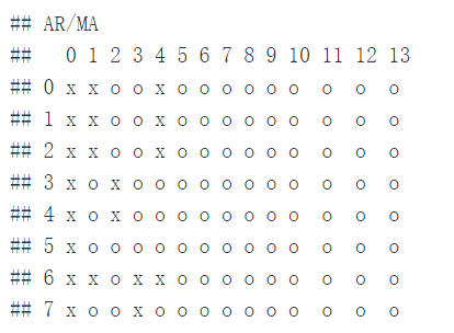
eacf函数
library(TSA)
eacf(ts)
MA建模
定阶
Acf函数
通过Acf函数, 看自相关系数, 取截尾处作为MA阶数
参数估计
Arima函数
fit=Arima(x1,order = c(2,0,0),method = c("CSS","CSS-ML", "ML"),include.drift = F)
#order=c(p,d,q), p是AR阶数, d是差分阶数, q是MA阶数
#include.drift = F 是不带有漂移项
#三个方法用一个, 如果不填默认是CSS-ML,
#如果估计值小于估计值误差的两倍, 则估计不显著,可以去掉
预测
forecast函数
forecast(fit,h=2,level=0.95) #h为预测步数, level为置信水平
AR建模
定阶
Pacf函数
通过Pacf函数, 看偏自相关系数, 取截尾处作为AR阶数
AR 过程参数估计
Arima函数
fit=Arima(x1,order = c(2,0,0),method = c("CSS","CSS-ML", "ML"),include.drift = F)
#order=c(p,d,q), p是AR阶数, d是差分阶数, q是MA阶数
#include.drift = F是不带有漂移项
#三个方法用一个, 如果不填默认是CSS-ML,
#如果估计值小于估计值误差的两倍, 则估计不显著,可以去掉
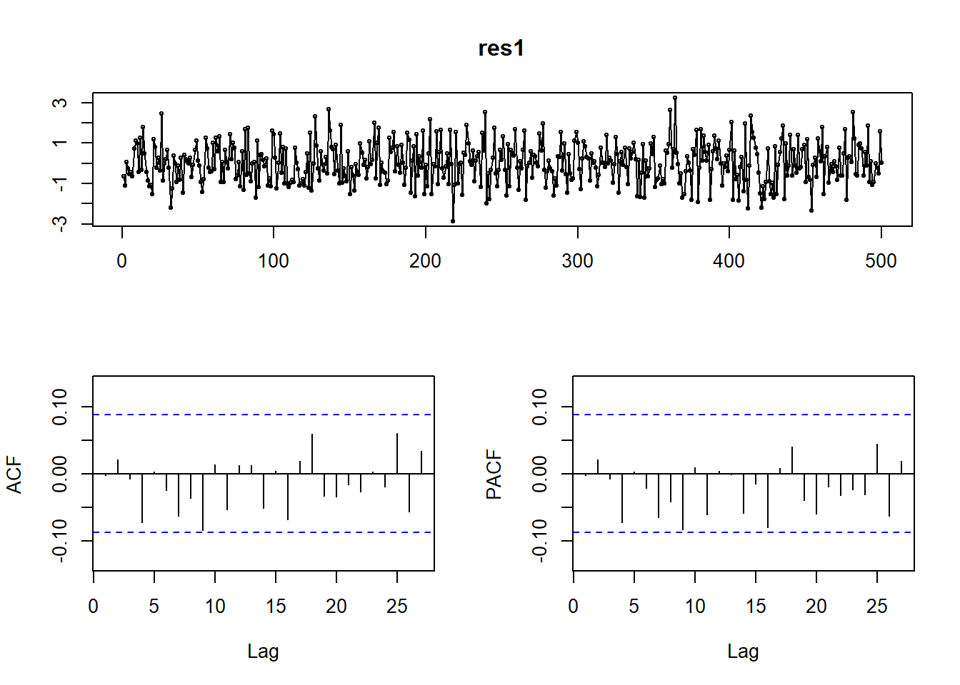
残差诊断
tsdisplay函数
tsdisplay(res)
Box.test函数
Box.test(res,lag=10,fitdf = p,type = "Ljung") #fitdf为AR阶数
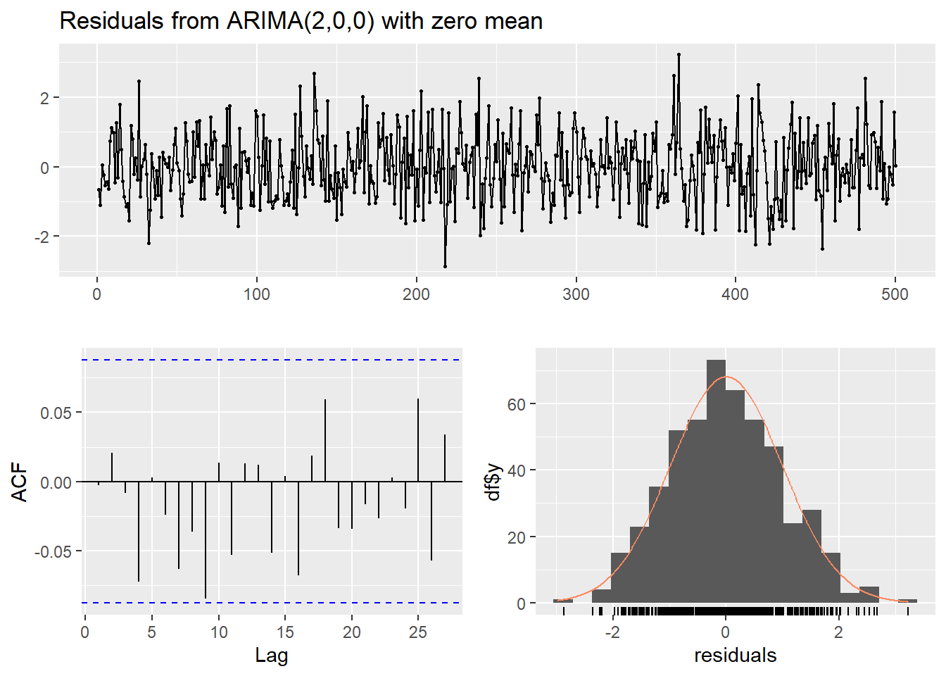
checkresiduals函数
checkresiduals(fit)#检验残差是不是白噪声, 输入对象是估计拟合
tsdiag模型诊断
tsdiag(fit)#, 输入对象是估计拟合
预测
forecast函数
forecast(fit,h=2,level=0.95) #h为预测步数, level为置信水平
异常值检验
tsoutliers异常值检验
outlier=tsoutliers(time_series) # 得出异常值的索引与对应的替换值
time_series[outlier$index]=outlier$replacements
混成检验
Box.test检验
Box.test(time_series,lag=?) lag是检验的自相关系数个数,检验序列是否为白噪声序列
差分
diff差分
ts.diff=diff(time_series,lag=1) #趋势差分
ts.diff=diff(time_series,lag=12) #季节差分
分解方法
-
mstlstl分解法
mstl函数可以不用指定参数,自动进行分解
fit_mstl <- mstl(time_series)

autoplot(fit_mstl[,"Remainder"]) #无规则项
autoplot(fit_mstl[,"Trend"]) #趋势项
autoplot(fit_mstl[,"Seasonal12"]) #季节项
-
stlstl分解法
fit_stl <- stl(x2,s.window = "periodic", t.window = 13)
#s.window,季节成分的窗宽,要么填"periodic",要么填大于7的奇数,必填
#t.window趋势成分的窗宽,需要奇数
autoplot(fit_stl)

autoplot(fit_stl$time.series[,"seasonal"]) #季节项
autoplot(fit_stl$time.series[,"trend"]) #趋势项
autoplot(fit_stl$time.series[,"remainder"]) #非规则项
-
seasX11方法
library(seasonal)
fit_x11 <- seas(time_series)
p + autolayer(fit_x11$data[,"seasonaladj"]) #季节调整后序列
autoplot(fit_x11$data[,"irregular"]) #剩余项无规则项的时序图
-
decompose经典分解法
经典分解法假设季节因子是恒定不变的,当序列较长时,这一假设可能并不合理
加法模型:
当周期性不随着趋势发生变化时,首选加法模型
当目标存在负值时,应选择加法模型
乘法模型:
周期随着随时发生变化时
经济数据,首选乘法模型(增长率、可解释)
fit_dc=decompose(time_series,type=c("additive", "multiplicative"))
# additive对应加法分解,multiplicative对应乘法分解
rand=fit_dc$random #经典分解剩余无规则项
趋势平滑
-
ma移动平均法趋势平滑(线性滤波的一个特例)
ma <- ma(time_series,order=3) #order是平滑窗宽,需要奇数
autoplot(time_series) + autolayer(ma)
-
filter线性滤波
fit <- filter(time_series,filter=c(1/4,1/2,1/4),sides = 2)
# filter通常应该是奇数长度, sides如果是1,则只用过去的值.如果是2,则以0为中心
autoplot(time_series) + autolayer(fit)
-
lm拟合线性趋势
t=time(time_series)
fit1=lm(time_series~t,data=y) #进行线性拟合
fitted1=ts(fit1$fitted.values) #将拟合好的已知点拟合结果变成时间序列
autoplot(time_series)+autolayer(fitted1) #展示原数据与拟合直线
-
lm拟合三次多项式趋势
t=time(time_series)
fit3=lm(time_series~t+I(t^2)+I(t^3)) #通过I()添加高次项拟合
fitted3=ts(fit3$fitted.values)
autoplot(time_series)+autolayer(fitted3)
-
loess局部多项式回归法
loess.fit <- loess(y ~ time(y)) #先进行拟合
loess.ts <- ts(loess.fit$fitted,start = 1,span=0.5) #把拟合值构成时间序列
#span控制光滑程度,越大越光滑
p+autolayer(loess.ts)
数据处理
-
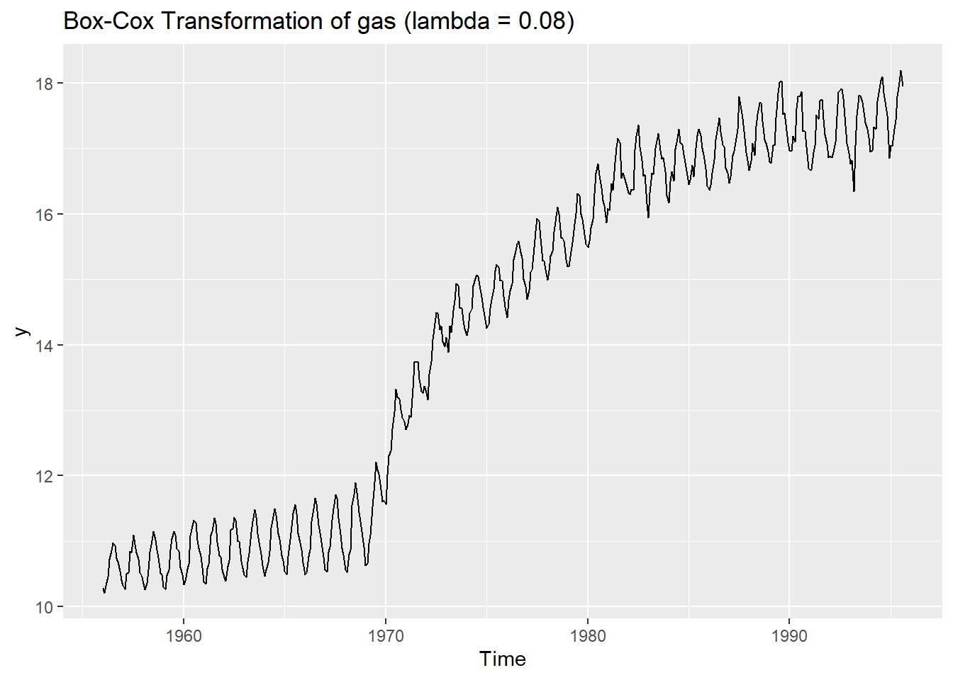
Box-Cox变换
autoplot(BoxCox(time_series,BoxCox.lambda(x))) #自动求Box-Cox参数
autoplot(BoxCox(time_series,0.1)) #自主设定Box-Cox参数, 参数越大,数值也越大
可视化
-
autolayer画布基础上增加曲线的函数
p+autolayer(object)
-
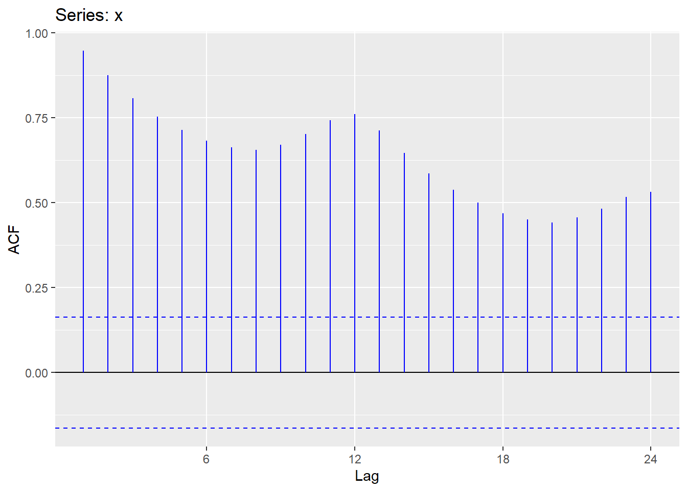
ggAcf相关图函数
ggAcf(time_series,col="blue") #直接出图显示
-
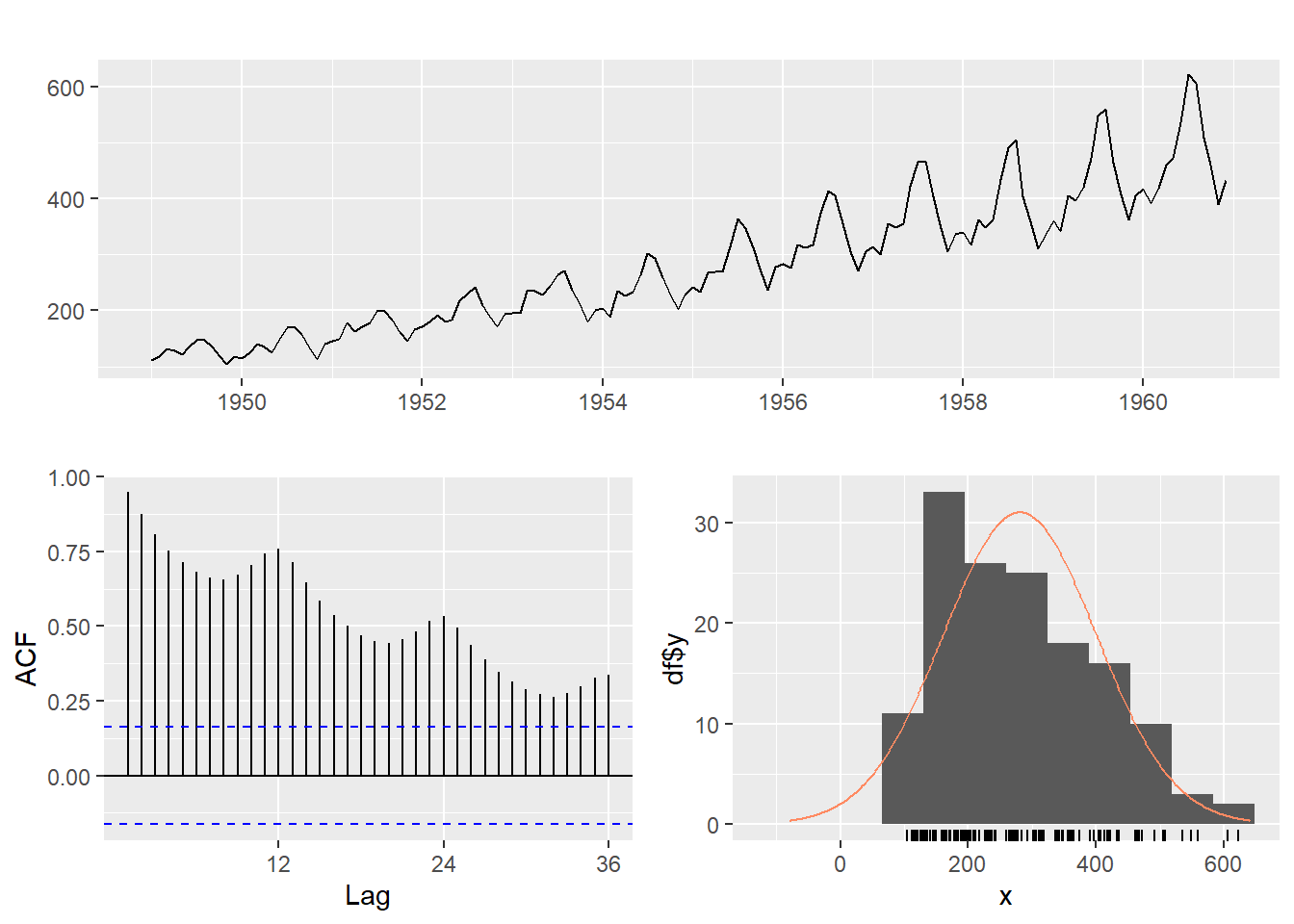
ggtsdisplay展示时间序列以及相关图与(偏相关图或其他)
ggtsdisplay(time_series)
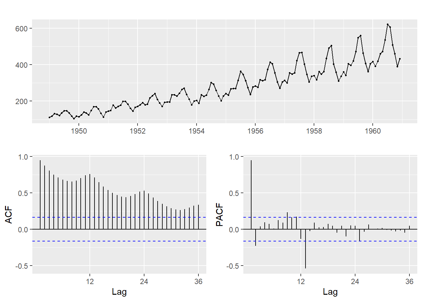
ggtsdisplay(time_series,plot.type = "histogram",points = F)
#plot.type是控制右下角的图的plot类型, points控制是否在时序图显示点
-
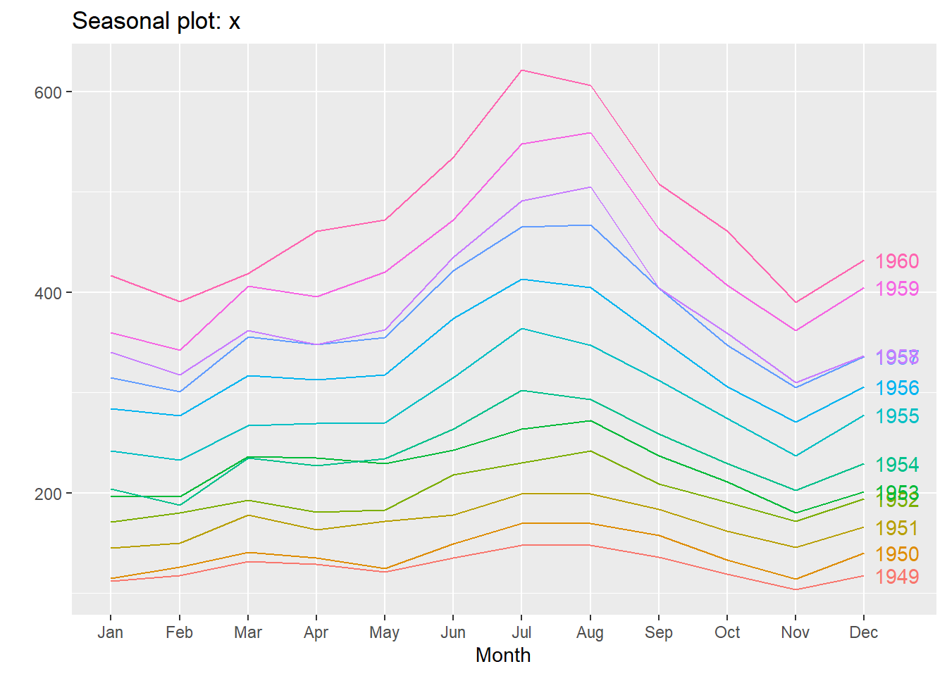
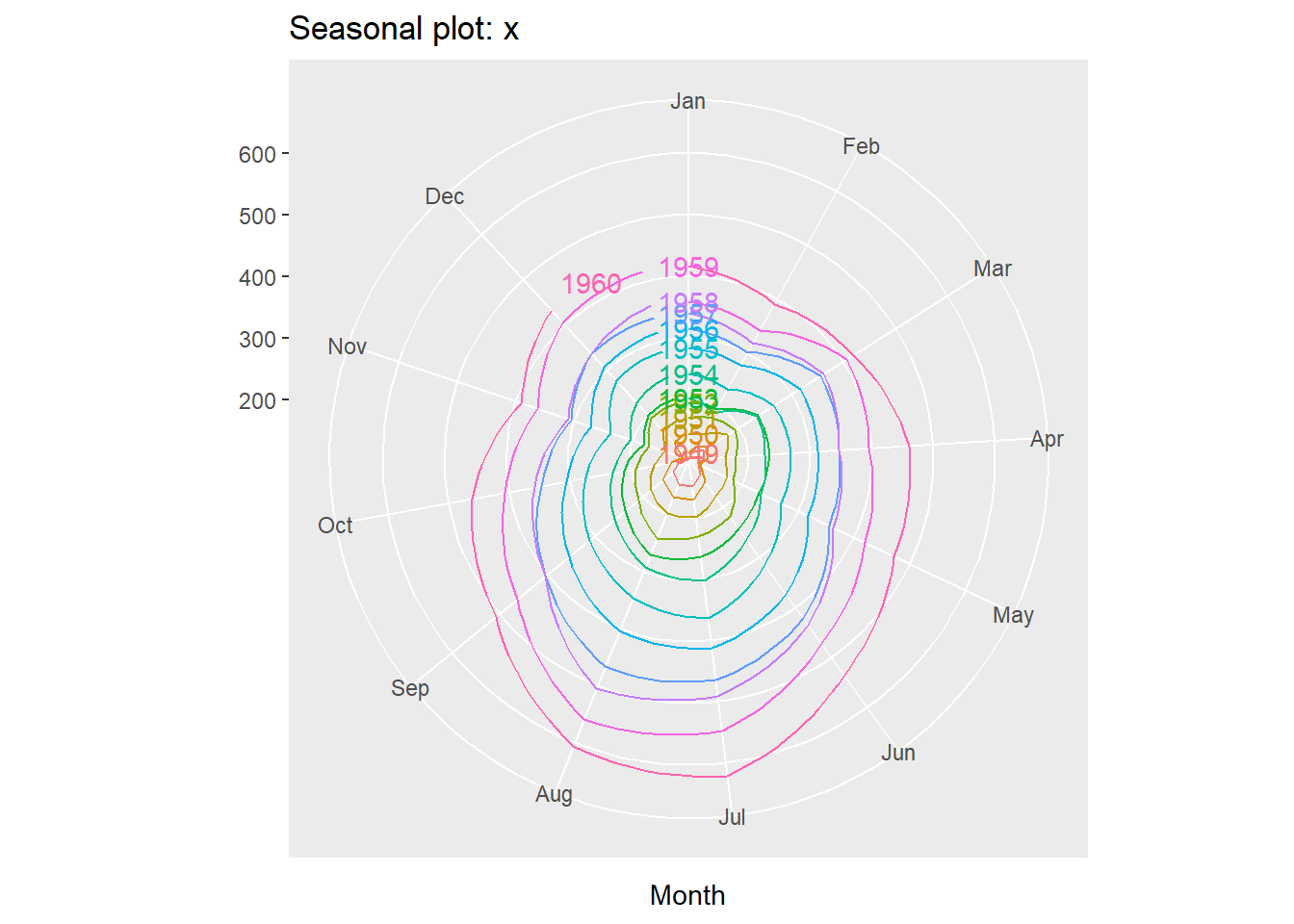
ggseasonplot季节图和雷达季节图
ggseasonplot(time_series,year.labels = T)
#ggseasonplot(time_series)#把year.labels设为TRUE才能把年份标到图右边的曲线里, 否则只能放到图外边的图例中
#year.labels.left设置为TRUE可以在曲线左边也显示年份
ggseasonplot(time_series,polar=TRUE,year.labels = T)
#将polar设置为TRUE可以将曲线变成极坐标形式显示
-
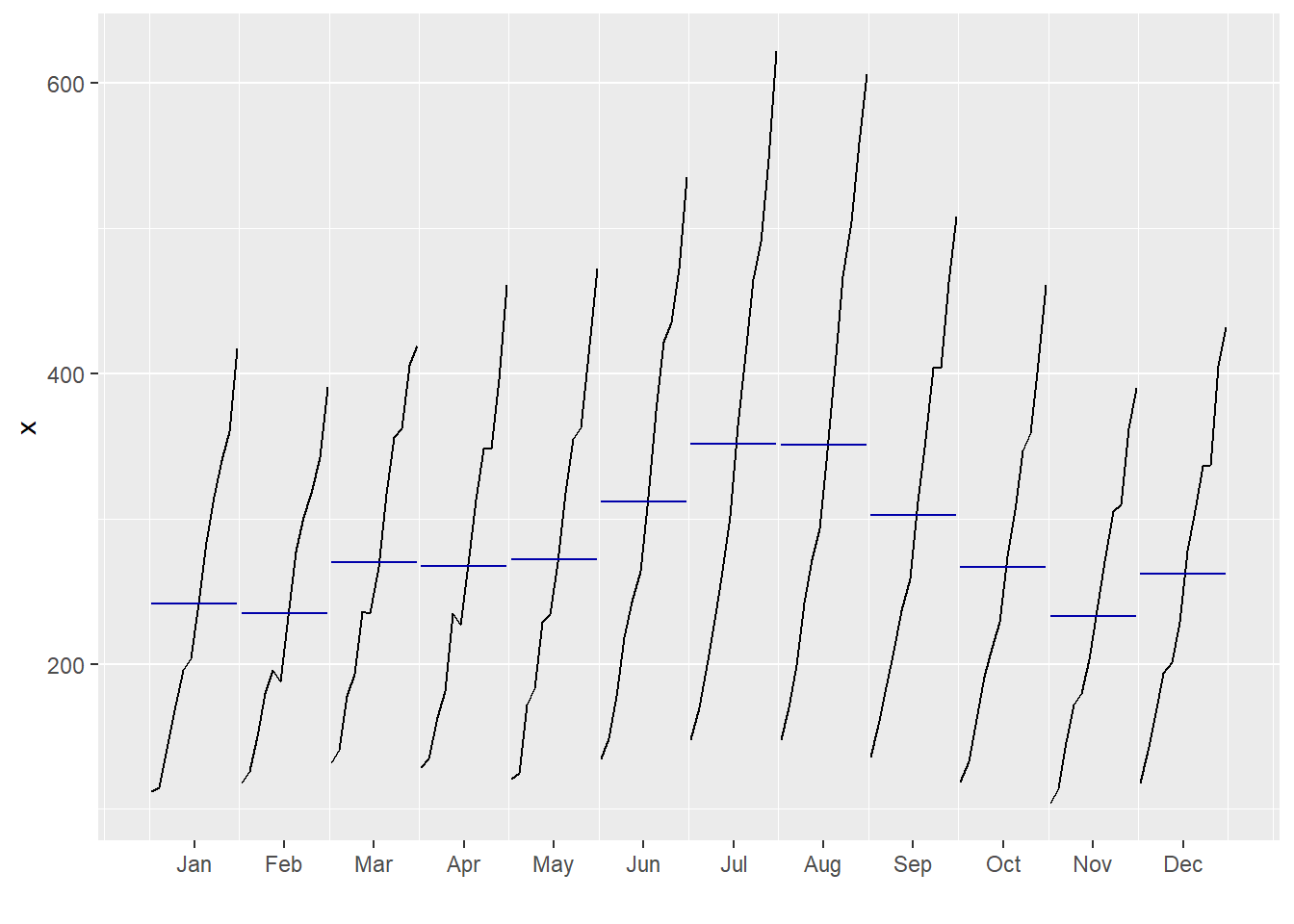
ggmonthplot季节子序列图
ggmonthplot(time_series) #直接出图
-
gglagplot延迟图(用于检测数据是否有随机性)
gglagplot(time_series, seasonal = FALSE, lags = 2, do.lines = FALSE)
#lags控制lag图个数,do.lines表示是否将点连线,seasonal如果是T,则彩色
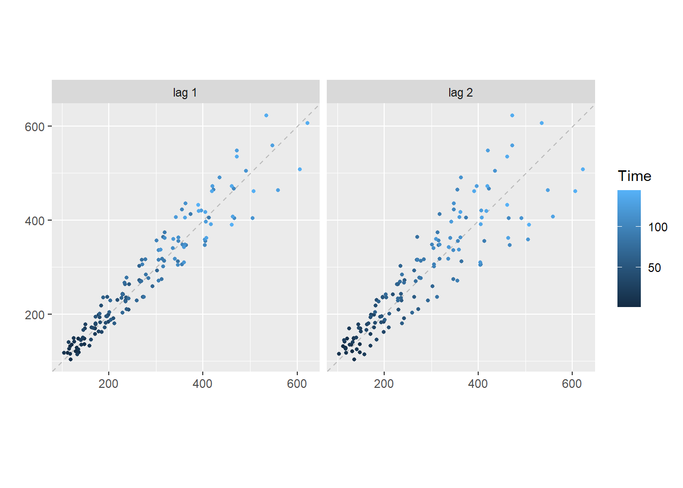
gglagplot(time_series, seasonal = TRUE, lags = 1, do.lines = T)
#lags控制lag图个数,do.lines表示是否将点连线,seasonal如果是T,则彩色
-
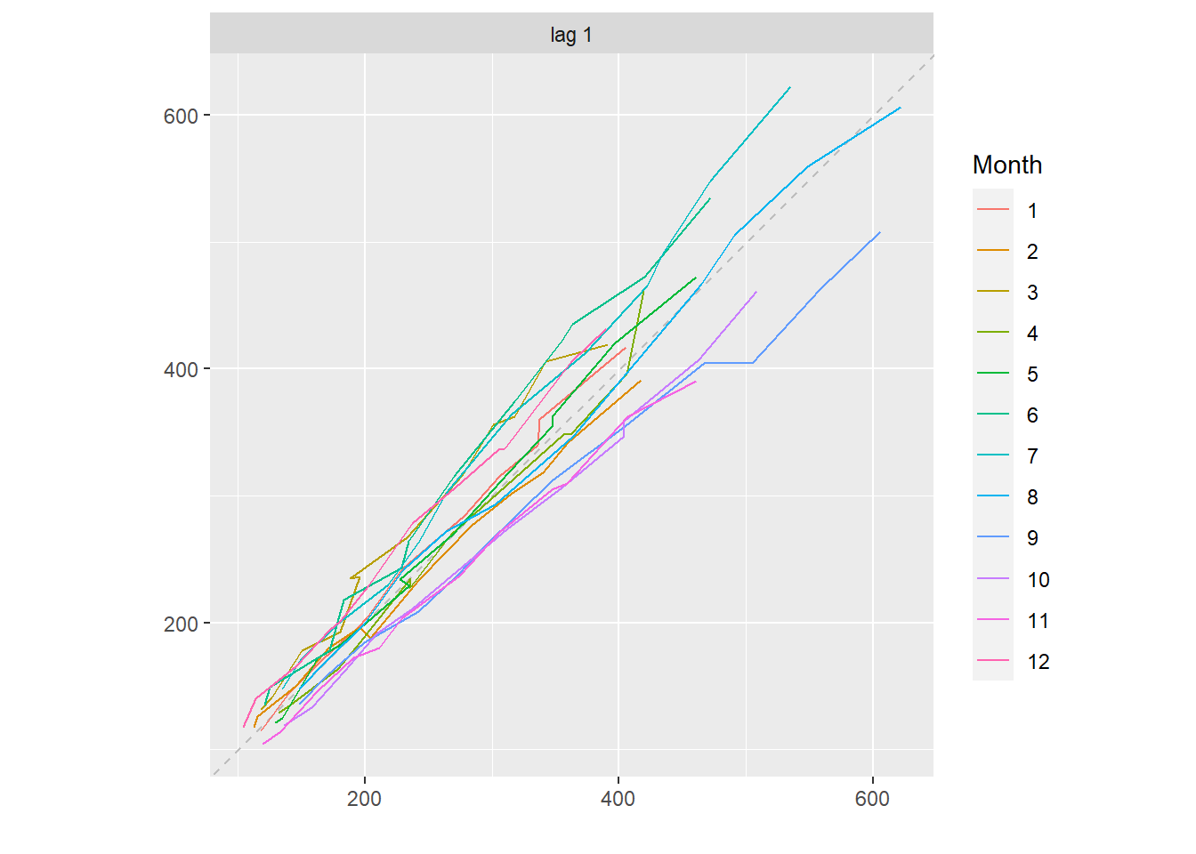
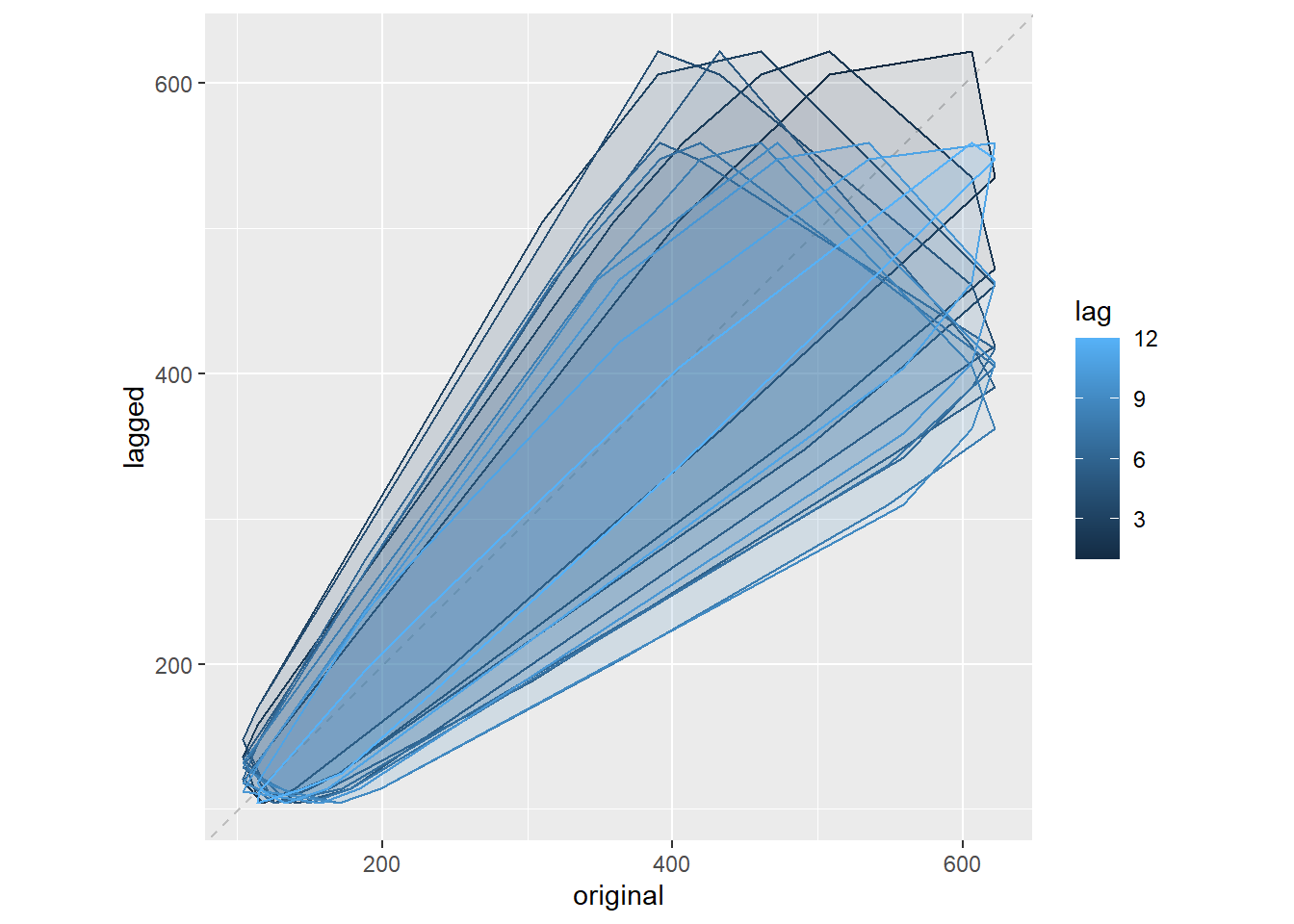
gglagchull延迟图(用于检测数据是否有随机性)
gglagchull(time_series)
-
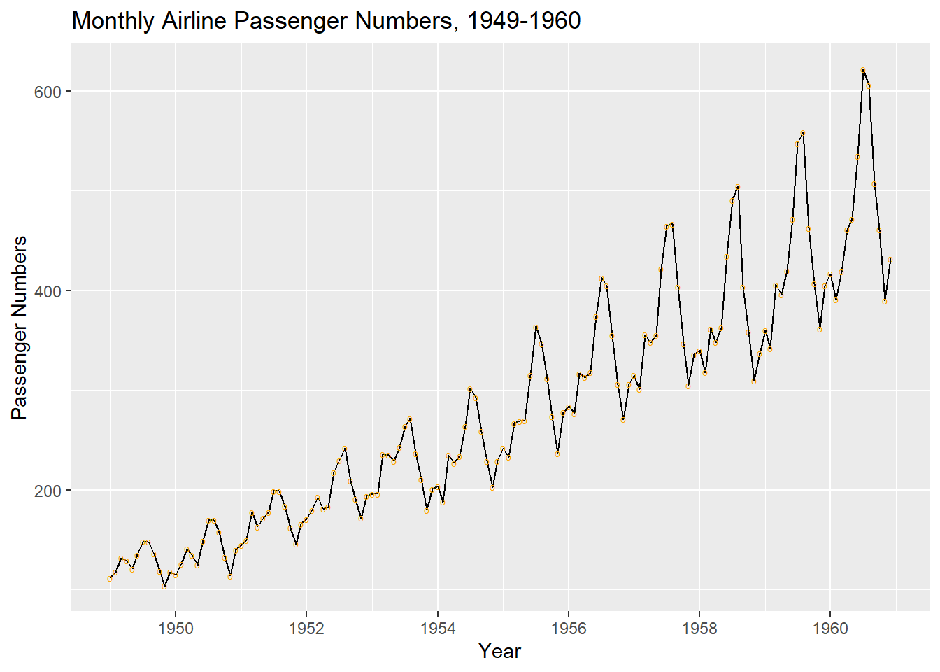
plot函数
plot(data_series,main="Title",ylab="value")
plot(data_series,type="o",main="title")#type指定数据点的形状
plot呈现的是空白背景的图
-
ggplot函数
ggplot(data)
#ggplot()括号内添加数据框可以建立初始画布

+ geom_point(aes(x=x1,y=y1),shape="o",col="orange")
#geom_point括号内添加通过aes()添加横纵坐标来添加散点, shape 和 col 分别控制点形状与颜色

+ geom_abline(intercept = beta_0, slope = beta_1, col="red")
#通过geom_abline添加直线,添加参数 lty=2 可以设置直线为虚线

+ggtitle("title") #通过ggtitle添加标题
+ylab("y") #添加y轴标签
+xlab("x") #添加x轴标签
-
autoplot函数
library(forecast)
library(ggplot2)
autoplot(data_series) + ggtitle("Title") + ylab="value"
autoplot生成灰色背景的有标度线的图

 浙公网安备 33010602011771号