卷积神经网络CNN（一）

　　对于CNN的学习，我先从代码部分入手，然后在学理论知识，两者相结合会达到豁然开朗的效果。

　　设置超参数

EPOCH = 1           # 训练整批数据多少次, 为了节约时间, 我们只训练一次
BATCH_SIZE = 50　　
LR = 0.001          # 学习率
DOWNLOAD_MNIST = True  # 如果你已经下载好了mnist数据就写上 False

　　下载数据集（可以是Mnist手写数据，也可以是Fashion Mnist）作为训练数据与测试数据

if not(os.path.exists('./mnist/')) or not os.listdir('./mnist/'):
    # not mnist dir or mnist is empyt dir
    DOWNLOAD_MNIST = True

train_data = torchvision.datasets.MNIST(
    root='./mnist/',
    train=True,                                     # 指定这是训练数据
　　　　
    transform=torchvision.transforms.ToTensor(),    # 将下载的数据转变为tensor形式的数据，并存储到train_data中
                                                    
    download=DOWNLOAD_MNIST,                        
)
train_loader = Data.DataLoader(dataset=train_data, batch_size=BATCH_SIZE, shuffle=True)

# 选择2000个样本进行测试
test_data = torchvision.datasets.MNIST(root='./mnist/', train=False)
test_x = torch.unsqueeze(test_data.test_data, dim=1).type(torch.FloatTensor)[:2000]/255.  
test_y = test_data.test_labels[:2000]

　　建立CNN模型：使用class来建立CNN模型，整体流程是卷积（Conv2d）-->激励函数（ReLU）-->池化，向下采样（MaxPooling）-->再来一遍-->接入全连接层（Linear）-->输出

　　【模型中的具体参数的理解见另一篇博客：卷积神经网络CNN（二） - Tzy0425 - 博客园 (cnblogs.com)】

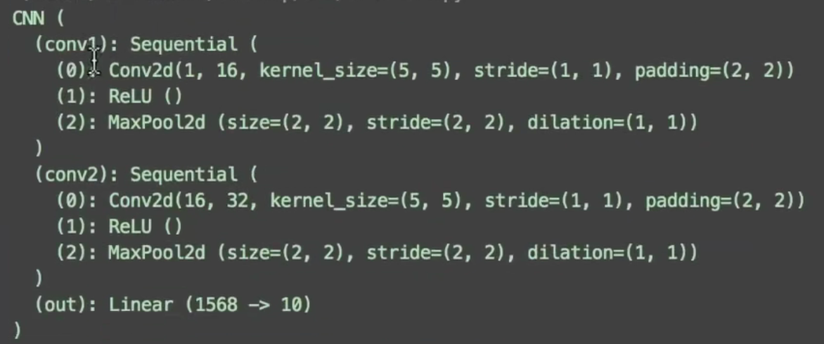
class CNN(nn.Module):
    def __init__(self):
        super(CNN, self).__init__()
        self.conv1 = nn.Sequential(         # 输入一张长宽为28的灰度图片，形状为(1, 28, 28)
            nn.Conv2d(
                in_channels=1,              # 输入图片的高度（本例中使用灰度图片，为1；若为RGB图片，则为3）
                out_channels=16,            # 经过过滤层扫描输出16个特征
                kernel_size=5,              # 过滤层的大小（长宽为5）
                stride=1,                   # 过滤层移动的步长
                padding=2,                  # 在输入的图片边缘填充2层像素
            ),                              # 输出的形状为(16, 28, 28)
            nn.ReLU(),                      # 激活函数
            nn.MaxPool2d(kernel_size=2),    # 相当于另一个过滤层，在每个2*2的范围选择一个最大值作为输出, 输出形状就被压缩为(16, 14, 14)
        )
        self.conv2 = nn.Sequential(         # 上一层的输出是这一层的输入，(16, 14, 14)
            nn.Conv2d(16, 32, 5, 1, 2),     # 这里的参数和上一层的参数含义完全一致，输出(32, 14, 14)
            nn.ReLU(),                      
            nn.MaxPool2d(2),                # 输出(32, 7, 7)
        )
        self.out = nn.Linear(32 * 7 * 7, 10)   # 连接Linear层，输出有10个分类，目前是3维数据，我们要展平为2维数据，在forward中进行

    def forward(self, x):
        x = self.conv1(x)
        x = self.conv2(x)
        x = x.view(x.size(0), -1)           # 最终的输出数据形式为：(batch_size, 32 × 7 × 7)
        output = self.out(x)
        return output, x                    # 返回x到可视化


cnn = CNN()
print(cnn)  # 打印cnn的结构

　　CNN的结构：

　　训练数据

for epoch in range(EPOCH):
    for step, (b_x, b_y) in enumerate(train_loader):   # enumerate表示输出时同时列出数据和数据下标

        output = cnn(b_x)[0]               
        loss = loss_func(output, b_y)   # cross entropy loss损失函数
        optimizer.zero_grad()           # 清空梯度
        loss.backward()                 # 反向传播，计算梯度
        optimizer.step()                # 更新参数

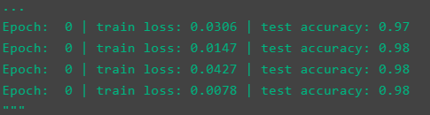
if step % 50 == 0:              # 每50步看一下训练效果，看一下预测的准确率为百分之多少
            test_output, last_layer = cnn(test_x)
            pred_y = torch.max(test_output, 1)[1].data.numpy()
            accuracy = float((pred_y == test_y.data.numpy()).astype(int).sum()) / float(test_y.size(0))
            print('Epoch: ', epoch, '| train loss: %.4f' % loss.data.numpy(), '| test accuracy: %.2f' % accuracy)

　　运行结果：

 

 

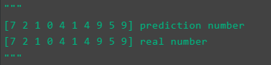
　　最后取10个数据，看预测的值是否正确

test_output, _ = cnn(test_x[:10])
pred_y = torch.max(test_output, 1)[1].data.numpy()
print(pred_y, 'prediction number')
print(test_y[:10].numpy(), 'real number')

　　运行结果：