机器学习—降维-特征选择6-3（PCA）

使用PCA对糖尿病数据集降维

主要步骤流程：

• 1. 导入包
• 2. 导入数据集
• 3. 数据预处理
  • 3.1 检测缺失值
  • 3.2 生成自变量和因变量
  • 3.3 拆分训练集和测试集
  • 3.4 特征缩放
• 4. 使用PCA降维
  • 4.1 使用 PCA 生成新的自变量
  • 4.2 验证PCA转换规则
    • 4.2.1 打印旧的自变量与新的自变量的转换系数
    • 4.2.2 增加转换系数的可读性
    • 4.2.3 检验X_train_pca的由来
  • 4.3 选择PCA个数
    • 4.3.1 打印 pca 的方差解释比率
    • 4.3.2 画出新的自变量的个数 VS 累计方差解释
  • 4.4 使用 PCA 降维
• 5. 构建逻辑回归模型
  • 5.1 使用原始数据构建逻辑回归模型
  • 5.2 使用降维后数据构建逻辑回归模型
• 6. 可视化PCA降维效果
  • 6.1 选择2个主成分
  • 6.2 可视化2个主成分

 

数据集链接：https://www.cnblogs.com/ojbtospark/p/16014512.html

 

1. 导入包

In [30]:

# 导入包
import numpy as np
import pandas as pd
import matplotlib.pyplot as plt

 

2. 导入数据集

In [31]:

# 导入数据集
dataset = pd.read_csv('pima-indians-diabetes.csv')
dataset

Out[31]:

	preg	plas	pres	skin	test	mass	pedi	age	class
0	6	148	72	35	0	33.6	0.627	50	1
1	1	85	66	29	0	26.6	0.351	31	0
2	8	183	64	0	0	23.3	0.672	32	1
3	1	89	66	23	94	28.1	0.167	21	0
4	0	137	40	35	168	43.1	2.288	33	1
...	...	...	...	...	...	...	...	...	...
763	10	101	76	48	180	32.9	0.171	63	0
764	2	122	70	27	0	36.8	0.340	27	0
765	5	121	72	23	112	26.2	0.245	30	0
766	1	126	60	0	0	30.1	0.349	47	1
767	1	93	70	31	0	30.4	0.315	23	0

768 rows × 9 columns

 

3. 数据预处理

3.1 检测缺失值

In [32]:

# 检测缺失值
null_df = dataset.isnull().sum()
null_df

Out[32]:

preg     0
plas     0
pres     0
skin     0
test     0
mass     0
pedi     0
age      0
class    0
dtype: int64

3.2 生成自变量和因变量

In [33]:

# 生成自变量和因变量
X = dataset.iloc[:,0:8].values
y = dataset.iloc[:,8].values

3.3 拆分训练集和测试集

In [34]:

# 拆分训练集和测试集
from sklearn.model_selection import train_test_split
X_train, X_test, y_train, y_test = train_test_split(X, y, test_size = 0.2, random_state = 1)
print(X_train.shape)
print(X_test.shape)
print(y_train.shape)
print(y_test.shape)

(614, 8)
(154, 8)
(614,)
(154,)

3.4 特征缩放

In [35]:

# 特征缩放
from sklearn.preprocessing import StandardScaler
sc_X = StandardScaler()
X_train = sc_X.fit_transform(X_train)
X_test = sc_X.transform(X_test)

 

4. 使用PCA降维

4.1 使用 PCA 生成新的自变量

In [92]:

# 使用 PCA 生成新的自变量
​
from sklearn.decomposition import PCA
pca = PCA(n_components = None) # 新的自变量的个数
X_train_pca = pca.fit_transform(X_train)
​
X_train_pca.shape

Out[92]:

(614, 8)

In [37]:

X_test_pca = pca.transform(X_test)

4.2 验证PCA转换规则

4.2.1 打印旧的自变量与新的自变量的转换系数

In [93]:

# 打印旧的自变量与新的自变量的转换系数
​
​
print('旧的自变量与新的自变量的转换系数是：\n', pca.components_)

旧的自变量与新的自变量的转换系数是：
 [[ 0.10403161  0.38834745  0.31001668  0.44761963  0.47331606  0.45153714
   0.29462719  0.16483609]
 [ 0.59215554  0.20495436  0.21141578 -0.3216619  -0.21416566 -0.08930935
  -0.08507664  0.63095277]
 [-0.01683682  0.40845294 -0.58777186 -0.24711536  0.25662924 -0.3200408
   0.5039637   0.06385032]
 [ 0.11775885 -0.52864182  0.10057944  0.06713469 -0.29647108  0.07267357
   0.77020171  0.0752341 ]
 [-0.51122484  0.3995761   0.33639051 -0.46774783 -0.35912494  0.2802682
   0.19022191 -0.05775928]
 [ 0.16516129  0.04357591 -0.60384046  0.03830138 -0.32007062  0.69929811
  -0.11174615  0.02797038]
 [-0.56399125 -0.0817524  -0.15954533  0.3307163  -0.11121765 -0.10982994
  -0.0800495   0.71383649]
 [ 0.13290372  0.43890844  0.01909041  0.54860634 -0.57668537 -0.31748978
   0.06072237 -0.2265163 ]]

4.2.2 增加转换系数的可读性

In [39]:

# 增加转换系数的可读性
old_columns = list(dataset)[:-1]
new_columns = ['pc' + str(i) + '_component' for i in range(X_train.shape[1])]
components_df = pd.DataFrame(pca.components_, columns = old_columns, index = new_columns)
components_df = components_df.T # 转置，增加可读性
print('打印旧的自变量与新的自变量的转换系数是：\n', components_df)

打印旧的自变量与新的自变量的转换系数是：
       pc0_component  pc1_component  pc2_component  pc3_component  \
preg       0.104032       0.592156      -0.016837       0.117759   
plas       0.388347       0.204954       0.408453      -0.528642   
pres       0.310017       0.211416      -0.587772       0.100579   
skin       0.447620      -0.321662      -0.247115       0.067135   
test       0.473316      -0.214166       0.256629      -0.296471   
mass       0.451537      -0.089309      -0.320041       0.072674   
pedi       0.294627      -0.085077       0.503964       0.770202   
age        0.164836       0.630953       0.063850       0.075234   

      pc4_component  pc5_component  pc6_component  pc7_component  
preg      -0.511225       0.165161      -0.563991       0.132904  
plas       0.399576       0.043576      -0.081752       0.438908  
pres       0.336391      -0.603840      -0.159545       0.019090  
skin      -0.467748       0.038301       0.330716       0.548606  
test      -0.359125      -0.320071      -0.111218      -0.576685  
mass       0.280268       0.699298      -0.109830      -0.317490  
pedi       0.190222      -0.111746      -0.080049       0.060722  
age       -0.057759       0.027970       0.713836      -0.226516  

4.2.3 检验X_train_pca的由来

In [40]:

print(X_train.shape)

(614, 8)

In [41]:

components = components_df.values
print(components.shape)

(8, 8)

In [42]:

# 检验x_train_pca的由来
verify_matrix = X_train.dot(components)

In [43]:

print(verify_matrix)

[[ 2.17984273  0.78840554 -0.29846515 ...  0.37864108 -0.23349737
   0.84660341]
 [ 0.91150409  1.01410624 -0.55536379 ...  1.65441098 -0.41829087
   0.80841226]
 [ 0.86350308  0.65153602 -1.23710744 ...  0.55528646  0.57655829
  -0.06548648]
 ...
 [ 0.70419613  2.7015353  -0.73401431 ...  1.01513112 -1.71268201
  -0.47664783]
 [ 0.39174323  0.39490219  0.17300319 ...  1.20502998 -1.12908868
   0.05638803]
 [ 0.61958733  1.26072012 -0.59500835 ...  0.32336925  0.27439521
   0.67636538]]

In [44]:

print(X_train_pca)

[[ 2.17984273  0.78840554 -0.29846515 ...  0.37864108 -0.23349737
   0.84660341]
 [ 0.91150409  1.01410624 -0.55536379 ...  1.65441098 -0.41829087
   0.80841226]
 [ 0.86350308  0.65153602 -1.23710744 ...  0.55528646  0.57655829
  -0.06548648]
 ...
 [ 0.70419613  2.7015353  -0.73401431 ...  1.01513112 -1.71268201
  -0.47664783]
 [ 0.39174323  0.39490219  0.17300319 ...  1.20502998 -1.12908868
   0.05638803]
 [ 0.61958733  1.26072012 -0.59500835 ...  0.32336925  0.27439521
   0.67636538]]

verify_matrix 和 X_train_pca一模一样

4.3 选择PCA个数

4.3.1 打印 pca 的方差解释比率

In [45]:

# 打印 pca 的方差解释比率
print('PCA的方差解释比率是：\n', pca.explained_variance_ratio_)

PCA的方差解释比率是：
 [0.26228657 0.21673495 0.13099609 0.10521342 0.09270677 0.08749259
 0.0539401  0.0506295 ]

4.3.2 画出新的自变量的个数 VS 累计方差解释

In [55]:

np.cumsum(pca.explained_variance_ratio_)

Out[55]:

array([0.26228657, 0.47902152, 0.61001761, 0.71523103, 0.80793781,
       0.8954304 , 0.9493705 , 1.        ])

In [58]:

# 画出新的自变量的个数 VS 累计方差解释
​
plt.plot([i for i in range(1, X_train.shape[1] + 1)], 
         np.cumsum(pca.explained_variance_ratio_), c='orange')
plt.xlabel('number of components')
plt.ylabel('cumulative explained variance')
h=6
plt.vlines(h, 0.2, 1, colors = "c", linestyles = "dashed")
plt.hlines(np.cumsum(pca.explained_variance_ratio_)[h-1], 8, 1,
           colors='c', linestyles='dashed')
plt.show()

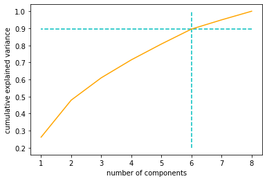
当降维后的自变量的个数是6时，能解释90%的方差。所以选择降维后自变量的个数是6。

4.4 使用 PCA 降维

In [19]:

# 使用 PCA 降维
pca = PCA(n_components = 6) # 6由上一步选出
X_train_pca = pca.fit_transform(X_train)
X_test_pca = pca.transform(X_test)
print(X_train_pca)

[[ 2.17984273  0.78840554 -0.29846515  0.32824425 -0.92432278  0.37864108]
 [ 0.91150409  1.01410624 -0.55536379  0.38428723 -0.87140245  1.65441098]
 [ 0.86350308  0.65153602 -1.23710744 -0.0095314  -1.31557169  0.55528646]
 ...
 [ 0.70419613  2.7015353  -0.73401431  0.90990109  0.32166808  1.01513112]
 [ 0.39174323  0.39490219  0.17300319 -0.59196727  1.96750054  1.20502998]
 [ 0.61958733  1.26072012 -0.59500835  1.37565681 -1.06613565  0.32336925]]

 

5. 构建逻辑回归模型

5.1 使用原始数据构建逻辑回归模型

In [20]:

# 构建模型
from sklearn.linear_model import LogisticRegression
classifier = LogisticRegression(penalty='l2', C=1,
                                class_weight='balanced', random_state = 0)
classifier.fit(X_train, y_train)

Out[20]:

LogisticRegression(C=1, class_weight='balanced', random_state=0)

In [21]:

# 预测测试集
y_pred = classifier.predict(X_test)

In [22]:

# 评估模型性能
from sklearn.metrics import accuracy_score
print(accuracy_score(y_test, y_pred))

0.7922077922077922

5.2 使用降维后数据构建逻辑回归模型

In [23]:

# 构建模型
classifier = LogisticRegression(penalty='l2', C=1, 
                                class_weight='balanced', random_state = 0)
classifier.fit(X_train_pca, y_train)

Out[23]:

LogisticRegression(C=1, class_weight='balanced', random_state=0)

In [24]:

# 预测测试集
y_pred = classifier.predict(X_test_pca)

In [25]:

# 评估模型性能
print(accuracy_score(y_test, y_pred))

0.7987012987012987

降维后，模型性能提升了0.006

 

6. 可视化PCA降维效果

可视化时，选择2个主成分。选择2个主成分信息有损失，这里目的仅仅是可视化

6.1 选择2个主成分

In [94]:

# 使用 PCA 降维
pca = PCA(n_components = 6)
X_train_pca = pca.fit_transform(X_train)

In [95]:

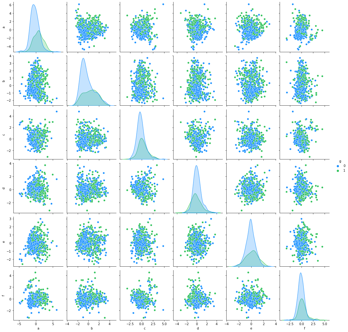
import seaborn as sns
ne=pd.concat([pd.DataFrame(X_train_pca),pd.DataFrame(y_train)],axis=1).reset_index(drop=True)
ne.columns = ['a', 'b', 'c', 'd', 'e','f','g']
antV = ['#1890FF', '#2FC25B']
sns.pairplot(ne,palette=antV,hue='g')

Out[95]:

<seaborn.axisgrid.PairGrid at 0x2d7f015f0a0>

 

6.2 可视化2个主成分

In [101]:

from matplotlib.colors import ListedColormap
X_set, y_set = X_train_pca, y_train
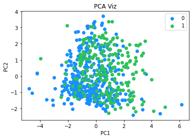
for i, j in enumerate(np.unique(y_set)):
    plt.scatter(X_set[y_set == j, 0], X_set[y_set == j, 1],
                color = ListedColormap(['#1890FF', '#2FC25B'])(i), label = j)
plt.title('PCA Viz')
plt.xlabel('PC1')
plt.ylabel('PC2')
plt.legend()
plt.show()

In [99]:

# 使用 PCA 降维
pca = PCA(n_components = 2)
X_train_pca = pca.fit_transform(X_train)
​
import seaborn as sns
ne=pd.concat([pd.DataFrame(X_train_pca),pd.DataFrame(y_train)],axis=1).reset_index(drop=True)
ne.columns = ['a', 'b','c']
antV = ['#1890FF', '#2FC25B']
sns.pairplot(ne,palette=antV,hue='c')

Out[99]:

<seaborn.axisgrid.PairGrid at 0x2d7eac74040>

 

 

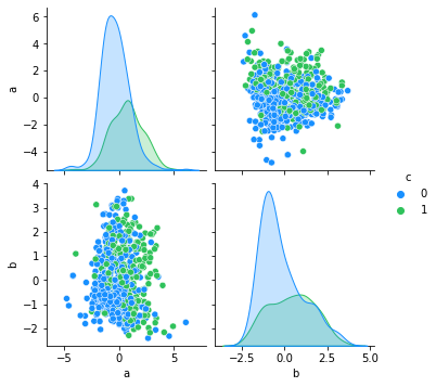
经过PCA降维，自变量由8个变为2个。

将降维后的2个主成分可视化，可以看到，如果以2个主成分训练逻辑回归模型，模型性能会较差，因为肉眼可见，2个类别之间没有明显的界限。