
机器学习—回归与分类4-1(决策树算法)
使用决策树预测德国人信贷风险
主要步骤流程:
- 1. 导入包
- 2. 导入数据集
- 3. 数据预处理
- 3.1 检测并处理缺失值
- 3.2 处理类别型变量
- 3.3 得到自变量和因变量
- 3.4 拆分训练集和测试集
- 3.5 特征缩放
- 4. 使用不同的参数构建决策树模型
- 4.1 模型1:构建决策树模型
- 4.1.1 构建模型
- 4.1.2 测试集做预测
- 4.1.3 评估模型性能
- 4.1.4 画出树形结构
- 4.2 模型2:构建决策树模型
- 4.1 模型1:构建决策树模型
In [1]:
# 导入包
import numpy as np
import pandas as pd
2. 导入数据集
In [2]:
# 导入数据集
data = pd.read_csv("german_credit_data.csv")
data
Out[2]:
3. 数据预处理
3.1 检测并处理缺失值
In [3]:
# 检测缺失值
null_df = data.isnull().sum() # 检测缺失值
null_df
Out[3]:
In [4]:
# 处理Saving accounts 和 Checking account 这2个字段
for col in ['Saving accounts', 'Checking account']: # 处理缺失值
    data[col].fillna('none', inplace=True) # none说明这些人没有银行账户
In [5]:
# 检测缺失值
null_df = data.isnull().sum()
null_df
Out[5]:
3.2 处理类别型变量
In [6]:
# 处理Job字段
print(data.dtypes)
In [7]:
data['Job'] = data['Job'].astype('object')
In [8]:
print(data.dtypes)
In [9]:
# 处理类别型变量
data = pd.get_dummies(data, drop_first = True)
data
Out[9]:
3.3 得到自变量和因变量
In [10]:
# 得到自变量和因变量
y = data['Risk_good'].values
data = data.drop(['Risk_good'], axis = 1)
x = data.values
3.4 拆分训练集和测试集
In [11]:
# 拆分训练集和测试集
from sklearn.model_selection import train_test_split
x_train, x_test, y_train, y_test = train_test_split(x, y, test_size = 0.2, random_state = 1)
print(x_train.shape)
print(x_test.shape)
print(y_train.shape)
print(y_test.shape)
3.5 特征缩放
In [12]:
# 特征缩放
from sklearn.preprocessing import StandardScaler
sc_x = StandardScaler()
x_train = sc_x.fit_transform(x_train)
x_test = sc_x.transform(x_test)
4. 使用不同的参数构建决策树模型
4.1 模型1:构建决策树模型
4.1.1 构建模型
In [23]:
# 使用不同的参数构建决策树模型
# 模型1:构建决策树模型(criterion = 'entropy', max_depth = 3, min_samples_leaf = 50)
from sklearn.tree import DecisionTreeClassifier
classifier = DecisionTreeClassifier(criterion = 'entropy', max_depth = 5, min_samples_leaf = 10, random_state = 0)
classifier.fit(x_train, y_train)
Out[23]:
4.1.2 测试集做预测
In [24]:
# 在测试集做预测
y_pred = classifier.predict(x_test)
4.1.3 评估模型性能
In [25]:
# 评估模型性能
from sklearn.metrics import accuracy_score
print(accuracy_score(y_test, y_pred))
In [26]:
from sklearn.metrics import confusion_matrix
print(confusion_matrix(y_test, y_pred))
In [27]:
from sklearn.metrics import classification_report
print(classification_report(y_test, y_pred))
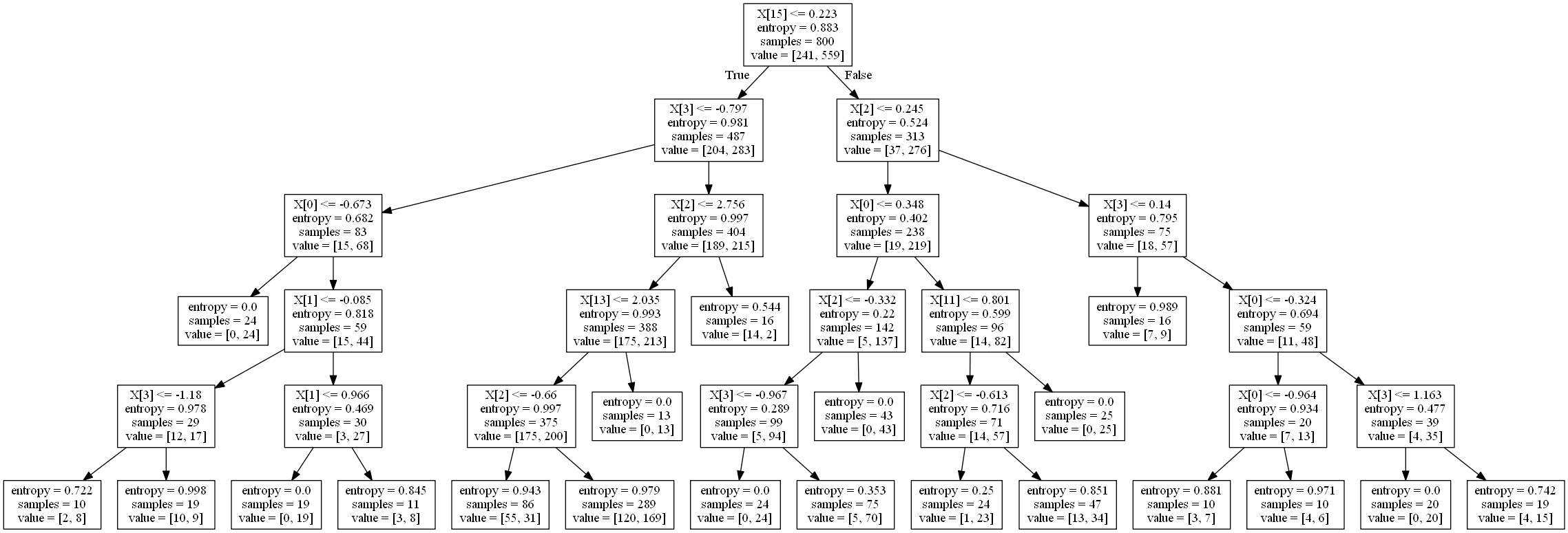
4.1.4 画出树形结构
准备工作:
- 安装graphviz库,使用命令 pip install graphviz
- 安装graphviz应用程序,并添加环境变量
In [28]:
# 生成.dot文件(在Jupyter Notebook中运行会报错,但是.dot文件却成功生成了。在控制台运行不会报错。)
from sklearn import tree
import graphviz
graphviz.Source(tree.export_graphviz(classifier, out_file='output.dot'))
Out[28]:
注:下面代码在Jupyter无法运行,需要在控制台运行
In [ ]:
'''
# 将 dot 文件转换成图片文件或pdf文件
dot -Tpng output.dot -o output.png # 转换成png文件
dot -Tpdf output.dot -o output.pdf # 转换成pdf文件
'''![]()
4.2 模型2:构建决策树模型
In [34]:
# 模型2:构建决策树模型(criterion = 'gini', max_depth = 9, min_samples_leaf = 10)
classifier = DecisionTreeClassifier(criterion = 'gini', max_depth = 5, min_samples_leaf = 10, min_samples_split=10, random_state = 0)
classifier.fit(x_train, y_train)
Out[34]:
In [35]:
# 在测试集做预测
y_pred = classifier.predict(x_test)
In [36]:
# 评估模型性能
print(accuracy_score(y_test, y_pred))
In [37]:
print(confusion_matrix(y_test, y_pred))
In [38]:
print(classification_report(y_test, y_pred))
结论: 由上面2个模型可见,不同超参数对模型性能的影响不同

 浙公网安备 33010602011771号