python程序设计(四):python与人工智能

python与人工智能

python机器学习

用KNN算法实现鸢尾花分类

数据处理

导库

import numpy as np
import pandas as pd
import matplotlib.pyplot as plt
from sklearn.datasets import load_iris#鸢尾花数据集
import seaborn as sns#也用来绘图
from sklearn.model_selection import train_test_split#用来划分训练集和测试你集
from sklearn.preprocessing import StandardScaler#标准化处理
from sklearn.neighbors import KNeighborsClassifier#KNN算法

导入数据,分析数据

iris=load_iris()
data=pd.DataFrame(iris.data)#得到data和target,都是一个numpy二维数组
target=pd.DataFrame(iris.target)
df=pd.concat((data,target),axis=1)#把data和target合并
df.columns=['sl','sw','pl','pw','target']#设置列名
df

	sl	sw	pl	pw	target
0	5.1	3.5	1.4	0.2	0
1	4.9	3.0	1.4	0.2	0
2	4.7	3.2	1.3	0.2	0
3	4.6	3.1	1.5	0.2	0
4	5.0	3.6	1.4	0.2	0
...	...	...	...	...	...
145	6.7	3.0	5.2	2.3	2
146	6.3	2.5	5.0	1.9	2
147	6.5	3.0	5.2	2.0	2
148	6.2	3.4	5.4	2.3	2
149	5.9	3.0	5.1	1.8	2

150 rows × 5 columns

target_names=iris.target_names#获取target标签,用于标志
target_names

array(['setosa', 'versicolor', 'virginica'], dtype='<U10')

df.corr()#列出比尔森相关系数

	sl	sw	pl	pw	target
sl	1.000000	-0.117570	0.871754	0.817941	0.782561
sw	-0.117570	1.000000	-0.428440	-0.366126	-0.426658
pl	0.871754	-0.428440	1.000000	0.962865	0.949035
pw	0.817941	-0.366126	0.962865	1.000000	0.956547
target	0.782561	-0.426658	0.949035	0.956547	1.000000

数据可视化

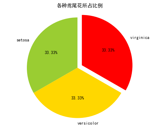
①饼图

plt.rcParams['font.sans-serif'] = ['SimHei']#用plt.rcParams设置字体
counts=df['target'].value_counts() #返回结果按频数从大到小排列
x=[counts.iloc[0],counts.iloc[1],counts.iloc[2]]
labels=[target_names[0],target_names[1],target_names[2]]
colors=['yellowgreen','gold','#FF0000']
explode=(0,0,0.1)
plt.pie(x,explode=explode,labels=labels,colors=colors,autopct="%1.2f%%",startangle=90)
plt.title('各种鸢尾花所占比例')#fontpreperties已弃用
plt.axis('equal')
plt.show()

②用seaborn库绘图

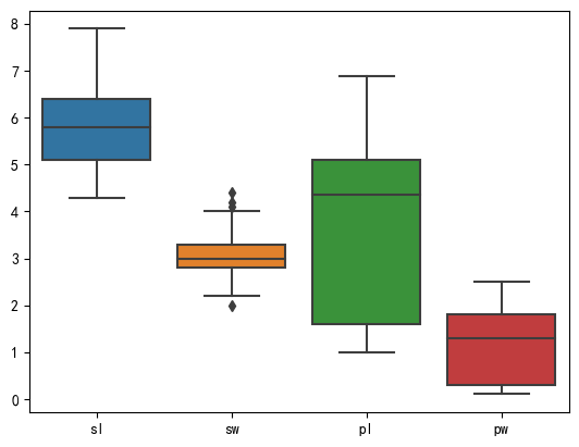
盒图

iloc切换,第一个参数表示行,:表示所有行,第二个参数表示列,:4=0:4也就是第0-3列

sns.boxplot(data=df.iloc[:,:4])
plt.show()
sns.boxplot(x=df['target'],y=df['sl'])
plt.show()

小提琴图

ax=sns.violinplot(data=df.iloc[:,:4])
ax.set_title('四个特征值的分布情况')
plt.show()

数据预处理

①分割训练集和测试集

x_train,x_test,y_train,y_test=train_test_split(data,target,test_size=0.25 ,
random_state=0)

有时还会分割出验证集

test_size=0.25 :指定测试集占25%,训练集就占75%
random_state=0 :指定了随机种子,这样每次产生的训练集和测试集元素固定
由于data,target均为DAtaFrame,所以x_train,x_test,y_train,y_test都是DataFrame,且y_train和y_test的秩为2

②对训练集和测试的特征数据进行标准化(标准化不一定是必须的)

ss=StandardScaler()
x_train=ss.fit_transform(x_train)#求x_train的均值和标准差,然后转换数据
x_test=ss.transform(x_test)

ss.transform 用上一步算得的x_train的均值和标准差,来对x_test数据进行标准化.

③定义模型,进行训练

knn=KNeighborsClassifier(n_neighbors=5)
knn.fit(x_train,y_train)
y_predict=knn.predict(x_test)
print(y_predict)

[2 1 0 2 0 2 0 1 1 1 2 1 1 1 1 0 2 1 0 0 2 1 0 0 2 0 0 1 1 0 2 1 0 2 2 1 0
 2]


c:\environment\python\lib\site-packages\sklearn\neighbors\_classification.py:207: DataConversionWarning: A column-vector y was passed when a 1d array was expected. Please change the shape of y to (n_samples,), for example using ravel().
  return self._fit(X, y)

提示了knnfit()的第二个参数要求是1个1维numpy数组,但传入的y_train是一个2维数组的DataFrame,可以使用y_train.values.ravel()

knn.fit(x_train,y_train.values.ravel())
y_predict=knn.predict(x_test)
print(y_predict)

[2 1 0 2 0 2 0 1 1 1 2 1 1 1 1 0 2 1 0 0 2 1 0 0 2 0 0 1 1 0 2 1 0 2 2 1 0
 2]

④结果评估

方法1:使用模型自带的评估函数进行准确性测评

print(knn.score(x_test,y_test))

0.9473684210526315

方法2:使用sklearn.metrics李的classification_report模块对预测结果做更详细的分析

from sklearn.metrics import classification_report
print(classification_report(y_test,y_predict,target_names=target_names))

              precision    recall  f1-score   support

      setosa       1.00      1.00      1.00        13
  versicolor       1.00      0.88      0.93        16
   virginica       0.82      1.00      0.90         9

    accuracy                           0.95        38
   macro avg       0.94      0.96      0.94        38
weighted avg       0.96      0.95      0.95        38

方法3:使用混淆矩阵查看分类结果

from sklearn.metrics import confusion_matrix
cm=confusion_matrix(y_test,y_predict)
print(cm)

[[13  0  0]
 [ 0 14  2]
 [ 0  0  9]]

把y_test,y_predict合并在一块观察

np.hstack((y_test.values,y_predict.reshape(-1,1)))

array([[2, 2],
       [1, 1],
       [0, 0],
       [2, 2],
       [0, 0],
       [2, 2],
       [0, 0],
       [1, 1],
       [1, 1],
       [1, 1],
       [2, 2],
       [1, 1],
       [1, 1],
       [1, 1],
       [1, 1],
       [0, 0],
       [1, 2],
       [1, 1],
       [0, 0],
       [0, 0],
       [2, 2],
       [1, 1],
       [0, 0],
       [0, 0],
       [2, 2],
       [0, 0],
       [0, 0],
       [1, 1],
       [1, 1],
       [0, 0],
       [2, 2],
       [1, 1],
       [0, 0],
       [2, 2],
       [2, 2],
       [1, 1],
       [0, 0],
       [1, 2]])

泰坦尼克号生还测试

导入数据

import pandas as pd
titanic=pd.read_csv(r'./titanic.txt')
titanic

	row.names	pclass	survived	name	age	embarked	home.dest	room	ticket	boat	sex
0	1	1st	1	Allen, Miss Elisabeth Walton	29.0000	Southampton	St Louis, MO	B-5	24160 L221	2	female
1	2	1st	0	Allison, Miss Helen Loraine	2.0000	Southampton	Montreal, PQ / Chesterville, ON	C26	NaN	NaN	female
2	3	1st	0	Allison, Mr Hudson Joshua Creighton	30.0000	Southampton	Montreal, PQ / Chesterville, ON	C26	NaN	(135)	male
3	4	1st	0	Allison, Mrs Hudson J.C. (Bessie Waldo Daniels)	25.0000	Southampton	Montreal, PQ / Chesterville, ON	C26	NaN	NaN	female
4	5	1st	1	Allison, Master Hudson Trevor	0.9167	Southampton	Montreal, PQ / Chesterville, ON	C22	NaN	11	male
...	...	...	...	...	...	...	...	...	...	...	...
1308	1309	3rd	0	Zakarian, Mr Artun	NaN	NaN	NaN	NaN	NaN	NaN	male
1309	1310	3rd	0	Zakarian, Mr Maprieder	NaN	NaN	NaN	NaN	NaN	NaN	male
1310	1311	3rd	0	Zenn, Mr Philip	NaN	NaN	NaN	NaN	NaN	NaN	male
1311	1312	3rd	0	Zievens, Rene	NaN	NaN	NaN	NaN	NaN	NaN	female
1312	1313	3rd	0	Zimmerman, Leo	NaN	NaN	NaN	NaN	NaN	NaN	male

1313 rows × 11 columns

查看数据shape大小

titanic.shape

(1313, 11)

查看前几行数据,可以发现,类型各异,有数值型,类别型,甚至还有缺失的数据
head(n):可以查看n行数据,缺省时默认为5行

titanic.head(10)

	row.names	pclass	survived	name	age	embarked	home.dest	room	ticket	boat	sex
0	1	1st	1	Allen, Miss Elisabeth Walton	29.0000	Southampton	St Louis, MO	B-5	24160 L221	2	female
1	2	1st	0	Allison, Miss Helen Loraine	2.0000	Southampton	Montreal, PQ / Chesterville, ON	C26	NaN	NaN	female
2	3	1st	0	Allison, Mr Hudson Joshua Creighton	30.0000	Southampton	Montreal, PQ / Chesterville, ON	C26	NaN	(135)	male
3	4	1st	0	Allison, Mrs Hudson J.C. (Bessie Waldo Daniels)	25.0000	Southampton	Montreal, PQ / Chesterville, ON	C26	NaN	NaN	female
4	5	1st	1	Allison, Master Hudson Trevor	0.9167	Southampton	Montreal, PQ / Chesterville, ON	C22	NaN	11	male
5	6	1st	1	Anderson, Mr Harry	47.0000	Southampton	New York, NY	E-12	NaN	3	male
6	7	1st	1	Andrews, Miss Kornelia Theodosia	63.0000	Southampton	Hudson, NY	D-7	13502 L77	10	female
7	8	1st	0	Andrews, Mr Thomas, jr	39.0000	Southampton	Belfast, NI	A-36	NaN	NaN	male
8	9	1st	1	Appleton, Mrs Edward Dale (Charlotte Lamson)	58.0000	Southampton	Bayside, Queens, NY	C-101	NaN	2	female
9	10	1st	0	Artagaveytia, Mr Ramon	71.0000	Cherbourg	Montevideo, Uruguay	NaN	NaN	(22)	male

使用info()查看各列的名称,非NaN数量,数据类型

titanic.info()

<class 'pandas.core.frame.DataFrame'>
RangeIndex: 1313 entries, 0 to 1312
Data columns (total 11 columns):
 #   Column     Non-Null Count  Dtype  
---  ------     --------------  -----  
 0   row.names  1313 non-null   int64  
 1   pclass     1313 non-null   object 
 2   survived   1313 non-null   int64  
 3   name       1313 non-null   object 
 4   age        633 non-null    float64
 5   embarked   821 non-null    object 
 6   home.dest  754 non-null    object 
 7   room       77 non-null     object 
 8   ticket     69 non-null     object 
 9   boat       347 non-null    object 
 10  sex        1313 non-null   object 
dtypes: float64(1), int64(2), object(8)
memory usage: 113.0+ KB

使用describe()查看数值列的统计描述,如果对非数值列也统计,则加上include="all"参数

titanic.describe()

	row.names	survived	age
count	1313.000000	1313.000000	633.000000
mean	657.000000	0.341965	31.194181
std	379.174762	0.474549	14.747525
min	1.000000	0.000000	0.166700
25%	329.000000	0.000000	21.000000
50%	657.000000	0.000000	30.000000
75%	985.000000	1.000000	41.000000
max	1313.000000	1.000000	71.000000

查看列标签

titanic.columns

Index(['row.names', 'pclass', 'survived', 'name', 'age', 'embarked',
       'home.dest', 'room', 'ticket', 'boat', 'sex'],
      dtype='object')

查看行索引

titanic.index

RangeIndex(start=0, stop=1313, step=1)

数据可视化

导入matplotlib库,用rcParams设置字体和负号

import matplotlib.pyplot as plt
plt.rcParams['font.sans-serif']=['SimHei']
plt.rcParams['axes.unicode_minus']=False

1,年龄和生还的关系

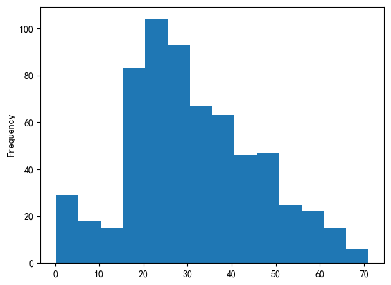
①观察所有乘客的年龄分布,绘制直方图

titanic['age'].plot(kind='hist',bins=14)#hist:类型为直方图,bins:设置分割的份
plt.show()

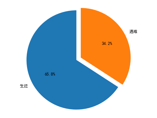
②绘制生还和遇难的比例饼图

x=titanic['survived'].value_counts()
plt.pie(x,labels=['生还','遇难'],autopct='%1.1f%%',startangle=90,explode=[0,0.1])
plt.axis('equal')#设置成正圆
plt.show()

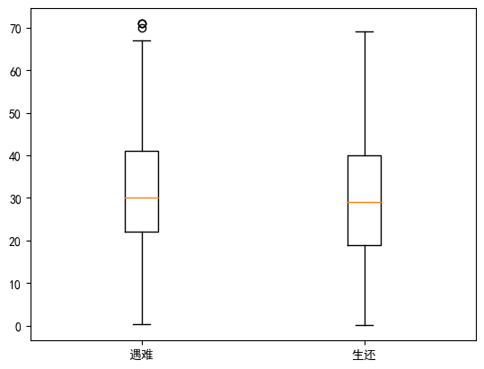
③绘制生还和遇难年龄分布的盒图

取满足条件的列的两种方法:
x_0=titanic[titanic['survived']0]['age'].dropna()
[titanic['survived']0]是满足survived==0的,['age']是取的列,.dropna():删除NaN

x_1=titanic.loc[titanic['survived']==1,'age'].dropna()
loc:用行列的名称 截取DataFrame数据
iloc:用矩阵下标 截取DataFrame数据

x_0=titanic[titanic['survived']==0]['age'].dropna()
x_1=titanic.loc[titanic['survived']==1,'age'].dropna()
plt.boxplot([x_0,x_1],labels=['遇难','生还'])
plt.show()

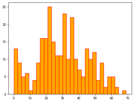
④所有生还者中年龄分布情况

x=titanic[titanic['survived']==1]['age'].dropna()
plt.hist(x,edgecolor='red',facecolor='orange',bins=30)
plt.show()

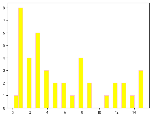
⑤15岁以下生还人员年龄分布

pandas和python不同,没有and not or,要用& | !

x=titanic[(titanic['survived']==1)&(titanic['age']<=15)]['age'].dropna()
plt.hist(x,edgecolor='pink',facecolor='yellow',bins=30)
plt.show()

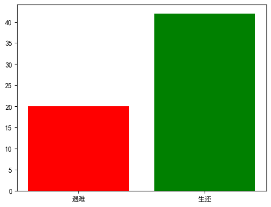
⑥绘制对比15岁以下遇难和生还的条形图

DataFrame.query()类似sql语句,且有and not or

plt.bar和plt.xtick设置刻度和刻度标签

x0=titanic.query('survived==0 and age<=15')['age']
x1=titanic.query('survived==1 and age<=15')['age']
plt.bar(x=0,height=len(x0),color='red')
plt.bar(x=1,height=len(x1),color='green')
plt.xticks([0,1],['遇难','生还'])
plt.show()

2.性别与生还的关系

groupby分析

titanic.groupby(['sex','survived']).count()

		row.names	pclass	name	age	embarked	home.dest	room	ticket	boat
sex	survived
female	0	156	156	156	44	54	48	5	1	4
	1	307	307	307	199	258	243	40	35	182
male	0	708	708	708	308	405	358	17	20	75
	1	142	142	142	82	104	105	15	13	86

遇难者中性别统计

x0=titanic[titanic['survived']==0]['sex'].value_counts()
x0

male      708
female    156
Name: sex, dtype: int64

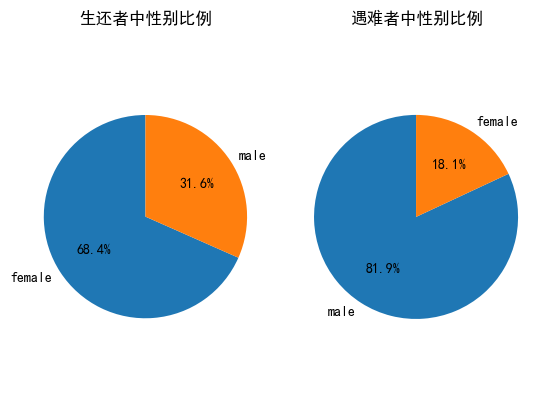
生还者,遇难者性别统计饼图

plt.subplot()设置多个图排列方式

x1=titanic[titanic['survived']==1]['sex'].value_counts()
plt.subplot(121)
plt.pie(x1,labels=x1.index,autopct='%1.1f%%',startangle=90)
plt.axis('equal')
plt.title('生还者中性别比例')
plt.subplot(122)
plt.pie(x0,labels=x0.index,autopct='%1.1f%%',startangle=90)
plt.title('遇难者中性别比例')
plt.axis('equal')
plt.show()

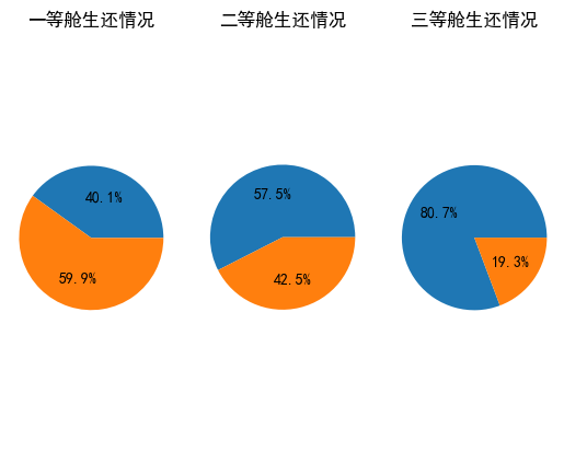
3,船舱等级和生还关系

创建交叉表,margins=True表示显示汇总信息

x=pd.crosstab(titanic.pclass,titanic.survived,margins=True)
x

survived	0	1	All
pclass
1st	129	193	322
2nd	161	119	280
3rd	574	137	711
All	864	449	1313

plt.subplot(131)
plt.pie(x.iloc[0, :2], labels = [' ',' '], autopct = '%1.1f%%')
plt.axis('equal')
plt.title('一等舱生还情况')
plt.subplot(132)
plt.pie(x.iloc[1, :2], labels = [' ',' '], autopct = '%1.1f%%')
plt.axis('equal')
plt.title('二等舱生还情况')
plt.subplot(133)
plt.pie(x.iloc[2, :2], labels = [' ',' '], autopct = '%1.1f%%')
plt.axis('equal')
plt.title('三等舱生还情况')
plt.show()

第二步,数据预处理,包括特征选择,填充nan值,数据特征化等

根据我们对事故的了解,sex,age,pclass这些都可能是决定幸免与否的关键因素

x=titanic[['pclass','age','sex']]
y=titanic['survived']
x.info()

<class 'pandas.core.frame.DataFrame'>
RangeIndex: 1313 entries, 0 to 1312
Data columns (total 3 columns):
 #   Column  Non-Null Count  Dtype  
---  ------  --------------  -----  
 0   pclass  1313 non-null   object 
 1   age     633 non-null    float64
 2   sex     1313 non-null   object 
dtypes: float64(1), object(2)
memory usage: 30.9+ KB

由info()的输出,拟设计如下几个数据预处理

1. age这个数据列只有633个non-null值,需要对null值进行补完
2. sex与pclass 两个数据列的值都是非数值型的,需要转为数值,用整数0/1 1/2/

首先补充age里的数据,使用平均数mean()或者中位数median()都是对模型偏离造成最小的策略

x=x.copy()

复制一份数据,否则会报错:A value is trying to be set on a copy of a slice from a DataFrame

x['age'].fillna(x['age'].mean(),inplace=True)

inplace=True表示原地修改

对补完的数据重新探查

x.info()

<class 'pandas.core.frame.DataFrame'>
RangeIndex: 1313 entries, 0 to 1312
Data columns (total 3 columns):
 #   Column  Non-Null Count  Dtype  
---  ------  --------------  -----  
 0   pclass  1313 non-null   object 
 1   age     1313 non-null   float64
 2   sex     1313 non-null   object 
dtypes: float64(1), object(2)
memory usage: 30.9+ KB

接着客舱等级,性别分别进行特征化

x.loc[x.sex=='male','sex']=0
x.loc[x.sex=='female','sex']=1
x.loc[x.pclass=='1st','pclass']=1
x.loc[x.pclass=='2nd','pclass']=2
x.loc[x.pclass=='3rd','pclass']=3

这里也可以用map函数

sex_dict={'male':0,'female':1}
x['sex']=x['sex'].map(sex_dict)

x.columns

Index(['pclass', 'age', 'sex'], dtype='object')

将数据分割为训练集和测试集

from sklearn.model_selection import train_test_split
x_train,x_test,y_train,y_test=train_test_split(x,y,test_size=0.25,random_state=33)

导入warning库,过滤可能的警告

import warnings
warnings.filterwarnings("ignore")

第三步,对模型进行训练,并预测,基本上是:导库-初始化-fit-predict四步

knn法

from sklearn.neighbors import KNeighborsClassifier
model=KNeighborsClassifier()
model.fit(x_train,y_train)
y_predict=model.predict(x_test)

其他实现算法:

#决策树
from sklearn.tree import DecisionTreeClassifier
model = DecisionTreeClassifier(criterion = 'entropy' )
model.fit(X_train, y_train)
y_predict = model.predict(X_test)
#随机森林法
from sklearn.ensemble import RandomForestClassifier
model = RandomForestClassifier()
model.fit(X_train, y_train)
y_predict = model.predict(X_test)
#线性分类器-逻辑回归分析
from sklearn.linear_model import LogisticRegression
model = LogisticRegression()
model.fit(X_train, y_train)
y_predict = model.predict(X_test)
#分类回归树CART
from sklearn.tree import DecisionTreeClassifier
model = DecisionTreeClassifier()
model.fit(X_train, y_train)
y_predict = model.predict(X_test)
#支持向量机SVM
from sklearn.svm import LinearSVC
model = LinearSVC()
model.fit(X_train, y_train)
y_predict = model.predict(X_test)
#朴素贝叶斯
from sklearn.naive_bayes import GaussianNB
model = GaussianNB()
model.fit(X_train, y_train)
y_predict = model.predict(X_test)

第四步结果评估

方法1:使用模型自带的评估函数

print(model.score(x_test,y_test))

0.7811550151975684

方法2:使用sklearn.metric里面的classification_report模块对预测结果做更详细的分析

from sklearn.metrics import classification_report
print(classification_report(y_test,y_predict,target_names=['died','survived']))

              precision    recall  f1-score   support

        died       0.78      0.90      0.83       202
    survived       0.79      0.59      0.68       127

    accuracy                           0.78       329
   macro avg       0.78      0.75      0.76       329
weighted avg       0.78      0.78      0.77       329

方法3:使用混淆矩阵查看分类效果

from sklearn.metrics import confusion_matrix
print(confusion_matrix(y_test,y_predict))

[[182  20]
 [ 52  75]]

一元线性回归

import numpy as np
import matplotlib.pyplot as plt
import mglearn
from sklearn.linear_model import LinearRegression
from sklearn.model_selection import train_test_split

X, y = mglearn.datasets.make_wave(n_samples=40)
X_train, X_test, y_train, y_test = train_test_split(X, y, random_state=42)
print(X.shape) 

(40, 1)

拟合x,y

lr = LinearRegression()
lr.fit(X_train, y_train)

LinearRegression()

In a Jupyter environment, please rerun this cell to show the HTML representation or trust the notebook.
On GitHub, the HTML representation is unable to render, please try loading this page with nbviewer.org.

输出模型参数

w are stored in coef_, b is stored in intercept_

print(lr.coef_) #coef_的类型为numpy.ndarray
print(lr.intercept_) #intercept_的类型为numpy.float64

[0.47954524]
-0.09847983994403892

分别用模型的score函数求训练集和测试集的拟合优度

print('Training set score:{:.3f}'.format(lr.score(X_train, y_train)))
print('test set score:{:.3f}'.format(lr.score(X_test, y_test)))

Training set score:0.653
test set score:0.773

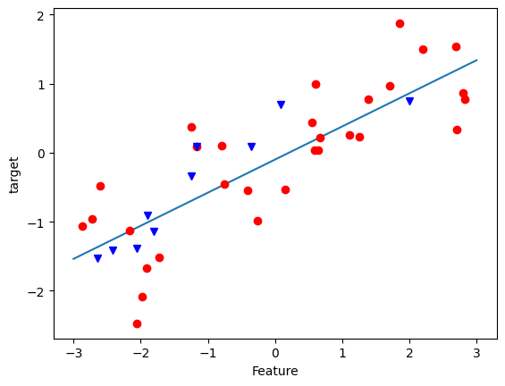
绘制样本和拟合直线

line = np.linspace(-3,3,1000).reshape(-1,1)
plt.plot(line[:,0], lr.predict(line))
plt.plot(X_train[:,0], y_train, 'o', c='r')
plt.plot(X_test[:,0], y_test, 'v', c='b')
plt.xlabel('Feature')
plt.ylabel('target')
plt.show()

波士顿房价预测

导库导数据

import numpy as np
import pandas as pd
import matplotlib.pyplot as plt
from sklearn.datasets import load_boston
from sklearn.model_selection import train_test_split
from sklearn.preprocessing import StandardScaler
from sklearn.linear_model import LinearRegression, SGDRegressor, Ridge
from sklearn.metrics import mean_squared_error
data = load_boston()

c:\environment\python\lib\site-packages\sklearn\utils\deprecation.py:87: FutureWarning: Function load_boston is deprecated; `load_boston` is deprecated in 1.0 and will be removed in 1.2.

    The Boston housing prices dataset has an ethical problem. You can refer to
    the documentation of this function for further details.

    The scikit-learn maintainers therefore strongly discourage the use of this
    dataset unless the purpose of the code is to study and educate about
    ethical issues in data science and machine learning.

    In this special case, you can fetch the dataset from the original
    source::

        import pandas as pd
        import numpy as np

        data_url = "http://lib.stat.cmu.edu/datasets/boston"
        raw_df = pd.read_csv(data_url, sep="\s+", skiprows=22, header=None)
        data = np.hstack([raw_df.values[::2, :], raw_df.values[1::2, :2]])
        target = raw_df.values[1::2, 2]

    Alternative datasets include the California housing dataset (i.e.
    :func:`~sklearn.datasets.fetch_california_housing`) and the Ames housing
    dataset. You can load the datasets as follows::

        from sklearn.datasets import fetch_california_housing
        housing = fetch_california_housing()

    for the California housing dataset and::

        from sklearn.datasets import fetch_openml
        housing = fetch_openml(name="house_prices", as_frame=True)

    for the Ames housing dataset.
  warnings.warn(msg, category=FutureWarning)

提示了波士顿房价的数据已经失效了,用新的数据:

import pandas as pd
import numpy as np
data_url = "http://lib.stat.cmu.edu/datasets/boston"
raw_df = pd.read_csv(data_url, sep="\s+", skiprows=22, header=None)
x = np.hstack([raw_df.values[::2, :], raw_df.values[1::2, :2]])
y = raw_df.values[1::2, 2]

import matplotlib.pyplot as plt
from sklearn.model_selection import train_test_split
from sklearn.preprocessing import StandardScaler
from sklearn.linear_model import LinearRegression, SGDRegressor, Ridge
from sklearn.metrics import mean_squared_error

X = data.data
y = data.target
X_train, X_test, y_train, y_test = train_test_split(X, y, test_size=0.25, random_state=0)
ss = StandardScaler()
X_train = ss.fit_transform(X_train)
X_test = ss.transform(X_test)

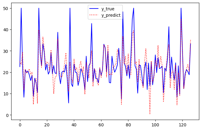
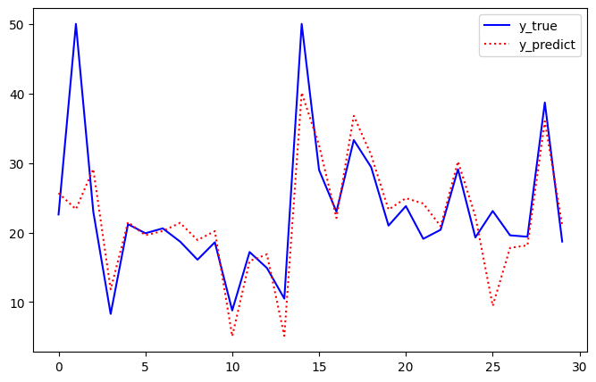
绘图函数

def plot_diff(y_test, y_pred):
 plt.figure(figsize=(8,5))
 plt.plot(y_test, 'b-', label='y_true')
 plt.plot(y_pred, 'r:', label='y_predict')
 plt.legend()
 plt.show()

(1)LinearRegression,线性回归(最小二乘法,用正规方程求解)

lr = LinearRegression()
lr.fit(X_train, y_train)
y_pred = lr.predict(X_test)
print(' MSE ', mean_squared_error(y_test, y_pred))
plot_diff(y_test, y_pred)
print(lr.coef_, lr.intercept_) 
print('Training set score:{:.3f}'.format(lr.score(X_train, y_train)))
print('test set score:{:.3f}'.format(lr.score(X_test, y_test)))

 MSE  29.78224509230234

[-0.97100092  1.04667838 -0.04044753  0.59408776 -1.80876877  2.60991991
 -0.19823317 -3.00216551  2.08021582 -1.93289037 -2.15743759  0.75199122
 -3.59027047] 22.6087071240106
Training set score:0.770
test set score:0.635

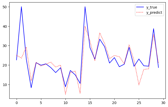
(2)SGDRegressor随机梯度下降回归,sklearn建议当样本数大于10万条时推荐用该算法

sg = SGDRegressor()
sg.fit(X_train, y_train)
y_pred = sg.predict(X_test)
print('SGD MSE ', mean_squared_error(y_test, y_pred))
plot_diff(y_test[:30], y_pred[:30])
print(sg.coef_, sg.intercept_) #输出模型参数
#分别计算训练集和测试集的拟合优度
print('Training set score:{:.3f}'.format(sg.score(X_train, y_train)))
print('test score:{:.3f}'.format(sg.score(X_test, y_test)))

SGD MSE  30.259089282498678

[-0.92911005  0.94412689 -0.27009504  0.65094279 -1.67117324  2.67070413
 -0.2352616  -2.90654782  1.52022938 -1.33845261 -2.13156707  0.75031598
 -3.57717671] [22.61254595]
Training set score:0.769
test score:0.630

什么时过拟合 和 欠拟合?

学习器把训练样本学得太好了的时候,可能把训练样本自身的一些特点当作了所有潜在的样本都会具有的一般性质,这样就会导致泛化能力下降,这种现象在机器学习中被称为"过拟合"(overfitting).
欠拟合(underfitting)是指学习能力低下,对训练样本的一般性质尚未学好

岭回归在线性回归的基础上添加了额外的约束条件,让w1,w2.....wn这些系数,尽可能变小,使每一个特征尽可能少地影响输出结果,即w系数都接近0,但不是0
约束条件通常是正则化,约束一个模型以避免过拟合,岭回归采用L2正则法,就是在损失函数后面添加L2范数

(3)岭回归Ridge--带有L2正则化的线性回归

rd = Ridge()
rd.fit(X_train, y_train)
y_pred = rd.predict(X_test)
print(' MSE ', mean_squared_error(y_test, y_pred))
plot_diff(y_test[:30], y_pred[:30])
print(rd.coef_, rd.intercept_)
print('Training set score:{:.3f}'.format(rd.score(X_train, y_train)))
print('test set score:{:.3f}'.format(rd.score(X_test, y_test)))

 MSE  29.853763334547615

[-0.96187481  1.02775462 -0.06861144  0.59814087 -1.77318401  2.6205672
 -0.20466821 -2.96504904  2.00091047 -1.85840697 -2.14955893  0.75175979
 -3.57350065] 22.6087071240106
Training set score:0.770
test set score:0.635

过拟合和岭回归

from mglearn.datasets import load_extended_boston
from sklearn.model_selection import train_test_split
from sklearn.linear_model import LinearRegression,Ridge
X, y = load_extended_boston()
X_train, X_test, y_train, y_test = train_test_split(X, y, test_size=0.25, random_state=40)

(1)线性回归LinearRegression

lr = LinearRegression()
lr.fit(X_train, y_train)
print(lr.coef_, lr.intercept_) 
print('Training set score:{:.3f}'.format(lr.score(X_train, y_train)))
print('test set score:{:.3f}'.format(lr.score(X_test, y_test)))

[-1.24333702e+02  8.51109172e-01 -8.78824412e+01  7.81825048e+00
 -4.06861380e+01  2.61890125e+01  5.47007747e+01 -6.90846361e+01
  5.01049890e+01  2.81858069e+01 -1.29429225e+01  4.81643468e+01
  6.04965107e+01  5.50775611e+01  1.81667676e+03  2.51073616e+02
  4.21555936e+02 -8.23756618e+01  2.68876268e+02 -1.07656749e+02
 -3.77037674e+02 -3.83383088e+02  3.51523319e+02 -7.35748233e+00
  2.67286847e+01  5.65099476e+01 -5.50667199e+00 -1.17926994e+01
 -1.28473035e+01 -2.76838844e+01 -2.87669962e+00 -3.85586219e-01
 -4.86621419e+00 -1.85513649e+01  2.19279307e+01 -8.67842854e+00
  1.76334139e+01 -2.61834116e+01  2.16356003e+01  2.99410370e+00
  1.04966826e+01  4.01265710e+01  1.63439867e+01  5.61180816e+01
 -1.91007517e+01  1.71622607e+01  4.10508880e+00  2.18656074e+01
  2.81273665e+00  7.81825048e+00 -1.18525934e+01 -3.62608172e+01
  3.05044951e+00  3.65981310e+01 -3.33277779e+00 -9.46859265e+00
 -9.73239134e+00  9.48538941e+00 -2.02269638e+01  2.06984374e+01
  2.40062595e+01 -2.30341997e+01  1.10903548e+02 -6.00556451e+00
  1.84622075e+01 -2.29697796e+01  2.29081600e+00  2.38457928e+01
  2.72633112e+01 -3.62438600e+01  2.99700977e+01 -2.37983636e+01
 -3.88143747e+01 -6.99662703e+00  1.07015056e+01 -7.44225841e+01
  4.91085514e+00 -6.78709407e+00  2.87845206e+01 -2.59067397e+01
 -2.42083666e+00 -3.87810818e+01 -2.28957639e+01  6.78634328e+01
 -2.08310147e+01 -2.57250801e+01 -5.43081961e+00 -3.02197012e+01
  4.93010816e+01 -7.63875125e+01  9.45133507e+01 -2.58006003e+01
 -7.40603658e+00 -1.00712059e+01 -1.24819910e+01  2.21603357e+01
 -2.13920836e+01 -2.88530760e+01  1.45291424e+00  1.89124871e+01
  5.70082642e+00 -9.67164307e+00 -2.30418042e+01 -1.06648201e+01] -17.07185865961382
Training set score:0.927
test set score:0.176

(2)岭回归Ridge

rd = Ridge()
rd.fit(X_train, y_train)
print(rd.coef_, rd.intercept_) 
print('Training set score:{:.3f}'.format(rd.score(X_train, y_train)))
print('test set score:{:.3f}'.format(rd.score(X_test, y_test)))

[-1.68841751e+00 -1.21756532e+00 -2.27229851e+00  8.29280456e-01
 -7.80743588e-02  8.01618677e+00 -2.42717943e-03 -4.69537735e+00
  3.64484835e+00 -1.77450946e+00 -1.84658519e+00  2.34935270e+00
 -2.79784030e+00 -1.03828380e+00  5.46354029e-03 -1.04992699e+00
  1.58455850e+00 -1.63046007e+00 -1.31404896e+00 -1.22931685e+00
 -3.40603690e-01 -1.96170505e+00 -1.69996969e+00 -1.54520138e+00
 -1.24905930e+00 -1.16408825e+00  1.86922579e+00 -1.84135671e+00
  2.15195000e+00  3.35085730e-01  3.44036564e+00 -1.95818731e+00
 -4.40322283e-01 -1.85312908e-01  3.52398000e-01  6.53546832e-01
 -1.00762321e+00 -1.77017868e+00  3.42121918e+00  1.40858792e+00
  8.78498660e-01 -3.91280661e+00  2.17738798e+00 -3.71752448e+00
  1.09951744e+00  2.54048858e+00 -1.16310771e+00 -5.71331629e-01
 -1.92919163e+00  8.29280456e-01 -4.89291341e+00 -3.66126587e+00
  1.33975269e+00 -1.17914224e+00  2.83125614e+00  3.21978680e+00
  3.94302777e-01  1.81255267e+00 -2.30766974e+00 -1.67414246e+00
 -3.53533236e+00 -2.17067231e+00 -9.25952604e-01 -2.49153483e+00
 -1.56089350e+00 -2.84270976e+00  1.55929616e+00 -1.87680529e+00
  1.49432569e+01 -3.73266046e-01  1.24079331e+00 -6.62933260e+00
 -7.51009416e+00 -4.29159411e+00  1.07477261e+01 -6.26321565e+00
  1.33172263e+00 -1.83931263e+00  3.61427066e+00  4.13554858e-01
 -1.69295163e+00 -1.99290831e+00 -3.25029990e+00  1.10791584e+00
 -1.59379257e+00 -2.74743398e+00 -7.72288993e-01 -3.81884579e+00
  3.77400765e-01  7.07738434e-01  7.60386326e-01  2.49785438e+00
  2.58562952e+00 -6.27464245e+00  1.51479963e+00  1.18250473e+00
 -1.16152937e+00 -6.38485861e+00  6.47776806e-01 -1.79770156e+00
 -1.71496657e+00 -1.00265130e+00 -5.90324030e+00  6.40531651e+00] 21.86084571054877
Training set score:0.834
test set score:0.860

Lasso回归是使用L1正则化的线性回归,相当于最小二乘法+L1范数

(3)Lasso回归

from sklearn.linear_model import Lasso
lasso = Lasso()
lasso.fit(X_train, y_train)
print(lasso.coef_, lasso.intercept_) 
print('Training set score:{:.3f}'.format(lasso.score(X_train, y_train)))
print('test set score:{:.3f}'.format(lasso.score(X_test, y_test)))

[-0.          0.         -0.          0.         -0.          0.
 -0.          0.         -0.         -0.         -0.          0.
 -0.32441098 -0.          0.         -0.          0.         -0.
 -0.         -0.         -0.         -0.         -0.         -0.
 -0.         -0.          0.          0.          0.          0.
  0.          0.          0.          0.          0.          0.
  0.          0.         -0.          0.         -0.         -0.
 -0.         -0.         -0.         -0.         -0.         -0.
 -0.          0.          0.          0.          0.          0.
  0.          0.          0.          0.          0.         -0.
 -0.         -0.         -0.         -0.         -0.         -0.
 -0.         -0.          0.          0.          0.         -0.
 -0.         -0.          0.         -0.         -0.         -0.
 -0.         -2.73694035 -0.73382069 -0.         -0.          0.
 -0.         -0.         -0.          0.         -0.         -0.
 -0.         -0.         -0.         -0.         -0.         -0.
 -0.         -0.         -0.         -0.         -0.          0.
 -0.         -0.        ] 23.777825319453992
Training set score:0.120
test set score:0.102

可以看到模型出现了欠拟合,实例化时Lasso()有正则化参数alpha,默认值alpha=1,alpha值越大则将w推向0的力度越大,而更低的alpha值将拟合出更复杂的模型,将alpha设置成0.01,max_iter=10000,iter_是迭代器迭代次数.Lasso因损失函数不是连续可导的,因此无法使用梯度下降法,常用坐标轴下降法或最小角回归法迭代求解

lasso = Lasso(alpha=0.01, max_iter=10000)
lasso.fit(X_train, y_train)
print(lasso.coef_, lasso.intercept_) 
print('Training set score:{:.3f}'.format(lasso.score(X_train, y_train)))
print('test set score:{:.3f}'.format(lasso.score(X_test, y_test)))

[ -0.          -0.          -0.           0.          -0.
   0.          -0.          -7.83175845   7.72112291   0.
  -0.           0.          -0.          -0.          -0.
  -0.           0.          -0.          -0.          -0.
  -0.          -7.57528476  -0.          -0.          -0.
  -0.           1.01619811  -0.           0.          -0.
   0.          -0.77056513   0.          -0.           0.
   0.          -0.          -0.           0.           0.
   0.          -0.           0.          -8.5544616    0.
   6.49229073  -0.          -0.          -0.           0.
  -4.86695189  -3.15397475   0.          -0.           0.
   7.74739138   0.           3.37036655  -0.          -1.01945969
  -4.67711816  -1.05909637  -0.          -0.          -0.
  -4.79229223   0.          -0.          26.4330005   -0.64282018
  -0.          -8.48483347 -11.5520677   -9.7055464   14.92670387
  -6.29599732  -0.          -0.29677602   4.57239306   0.
  -0.27696565  -2.111057    -0.96785033   0.          -0.
  -0.           0.          -0.           0.           0.
   0.           0.           0.45673343  -6.53072993   1.99027172
   0.           0.         -16.54235847   0.           0.
  -0.          -0.          -8.50513944   7.61285648] 20.64902255263751
Training set score:0.841
test set score:0.882

信用卡欺诈检测

logistic回归是机器学习中常用的二分类方法之一.虽然被称为回归模型,但是处理分类问题,它的本质是一个线性模型加上一个映射函数Sigmoid,将任意的输入映射到了[0,1]区间,从而完成了由值到概率的转换,概率值大于0.5的数据被分入1类

import numpy as np
import pandas as pd
import matplotlib.pyplot as plt
from sklearn.preprocessing import StandardScaler
from sklearn.linear_model import LogisticRegression
from sklearn.model_selection import train_test_split
from sklearn.metrics import classification_report

(1)读取数据,搜索数据

data = pd.read_csv("./creditcard.csv")
data.head()

	Time	V1	V2	V3	V4	V5	V6	V7	V8	V9	...	V21	V22	V23	V24	V25	V26	V27	V28	Amount	Class
0	0.0	-1.359807	-0.072781	2.536347	1.378155	-0.338321	0.462388	0.239599	0.098698	0.363787	...	-0.018307	0.277838	-0.110474	0.066928	0.128539	-0.189115	0.133558	-0.021053	149.62	0
1	0.0	1.191857	0.266151	0.166480	0.448154	0.060018	-0.082361	-0.078803	0.085102	-0.255425	...	-0.225775	-0.638672	0.101288	-0.339846	0.167170	0.125895	-0.008983	0.014724	2.69	0
2	1.0	-1.358354	-1.340163	1.773209	0.379780	-0.503198	1.800499	0.791461	0.247676	-1.514654	...	0.247998	0.771679	0.909412	-0.689281	-0.327642	-0.139097	-0.055353	-0.059752	378.66	0
3	1.0	-0.966272	-0.185226	1.792993	-0.863291	-0.010309	1.247203	0.237609	0.377436	-1.387024	...	-0.108300	0.005274	-0.190321	-1.175575	0.647376	-0.221929	0.062723	0.061458	123.50	0
4	2.0	-1.158233	0.877737	1.548718	0.403034	-0.407193	0.095921	0.592941	-0.270533	0.817739	...	-0.009431	0.798278	-0.137458	0.141267	-0.206010	0.502292	0.219422	0.215153	69.99	0

5 rows × 31 columns

data.isnull().values.sum()

0

绘制条形图

count_classes = pd.value_counts(data['Class'], sort = True).sort_index()
print(count_classes)

0    284315
1       492
Name: Class, dtype: int64

count_classes.plot(kind = 'bar', title='Fraud class histogram', rot=360) 
plt.show()

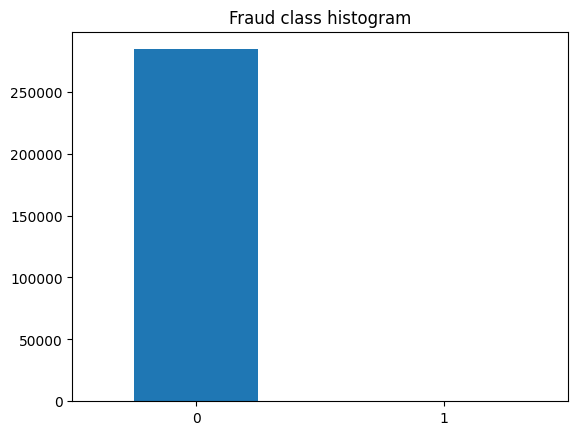
可以看到,由于数据量差距特别大,导致1的条形图无法显示

(2)数据的预处理

采样,确定建模数据.由于交易类型分布不平衡,不能简单粗暴地将原始数据切分成训练集和测试集.一种想法是:按标签为1的样本的样本数对标签为0的样本集进行1:1随机采样确定将来参与建模的全部样本,即随机下采用法

n = len(data[data.Class == 1])
indices_of_1 = np.array(data[data.Class == 1].index) 
indices_of_0 = data[data.Class == 0].index 
indices_of_0 = np.random.choice(indices_of_0, n, replace = False) 
indices = np.concatenate([indices_of_1,indices_of_0], axis=0) 
under_sample_data = data.iloc[indices,:] 
X_undersample = under_sample_data.loc[:,under_sample_data.columns != 'Class']
y_undersample = under_sample_data['Class']

划分训练集和测试集

X_train, X_test, y_train, y_test = train_test_split(X_undersample, y_undersample,
test_size=0.3, random_state=0) 

对Amount特征进行标准化

X_train = X_train.copy()
X_test = X_test.copy()
ss = StandardScaler()
X_train['normAmount'] = ss.fit_transform(X_train['Amount'].values.reshape(-1,1))
X_test['normAmount'] = ss.transform(X_test['Amount'].values.reshape(-1,1))
X_train = X_train.drop(['Time', 'Amount'], axis=1)
X_test = X_test.drop(['Time', 'Amount'], axis=1)
print(X_train)

              V1        V2        V3        V4        V5        V6        V7  \
6870   -1.863756  3.442644 -4.468260  2.805336 -2.118412 -2.332285 -4.261237   
150791  2.214237 -0.792902 -1.473319 -0.910354 -0.099301 -0.165655 -0.668552   
29464   1.213589 -0.741135  0.406263 -0.483767 -1.292866 -1.229874 -0.366938   
214775 -0.395582 -0.751792 -1.984666 -0.203459  1.903967 -1.430289 -0.076548   
149145 -2.405580  3.738235 -2.317843  1.367442  0.394001  1.919938 -3.106942   
...          ...       ...       ...       ...       ...       ...       ...   
218882 -6.650873 -5.166471  0.630071  1.977026  7.226284 -4.745045 -2.538954   
79536  -0.264869  3.386140 -3.454997  4.367629  3.336060 -2.053918  0.256890   
193748  2.313852 -1.447755 -1.107011 -1.572196 -1.228872 -0.615661 -1.194617   
84981  -0.775805  0.699239  2.156244 -0.505637 -0.285467 -0.753034  0.425022   
130031  1.485722 -0.329184 -0.650416 -1.049783  0.040445 -0.400925 -0.113134   

               V8        V9       V10  ...       V20        V21       V22  \
6870     1.701682 -1.439396 -6.999907  ...  0.360924   0.667927 -0.516242   
150791  -0.078229  0.966791  0.590159  ... -0.135084  -0.194810 -0.403193   
29464   -0.299762 -0.834289  0.599360  ...  0.261264   0.380608  0.852311   
214775  -0.992260  0.756307  0.217630  ... -1.027716   1.377515  2.151787   
149145 -10.764403  3.353525  0.369936  ... -2.140874  10.005998 -2.454964   
...           ...       ...       ...  ...       ...        ...       ...   
218882  -1.327611  1.026117  1.740803  ... -4.302659  -1.376437  0.010657   
79536   -2.957235 -2.855797 -2.808456  ...  0.482513  -1.394504 -0.166029   
193748  -0.075333 -0.943735  1.627065  ... -0.559194  -0.198388 -0.157568   
84981    0.071048 -0.089360 -0.633079  ...  0.138920  -0.085608 -0.291283   
130031  -0.223569 -1.421063  0.839325  ...  0.153764   0.172964  0.429903   

             V23       V24       V25       V26       V27       V28  normAmount  
6870   -0.012218  0.070614  0.058504  0.304883  0.418012  0.208858   -0.437003  
150791  0.201311 -0.011091 -0.079658 -0.375434 -0.079145 -0.079314   -0.377512  
29464  -0.194582  0.768330  0.573438 -0.071189 -0.012877  0.032184   -0.024683  
214775  0.189225  0.772943 -0.872443 -0.200612  0.356856  0.032113   -0.438240  
149145  1.684957  0.118263 -1.531380 -0.695308 -0.152502 -0.138866   -0.413087  
...          ...       ...       ...       ...       ...       ...         ...  
218882 -3.912938  0.437714  0.691167 -0.355594  0.612076 -0.184440   -0.284843  
79536  -1.452081 -0.251815  1.243461  0.452787  0.132218  0.424599   -0.437003  
193748  0.293418  0.600750 -0.222054 -0.181151 -0.004996 -0.050555   -0.401069  
84981  -0.099654  0.393402  0.298088  0.259466  0.167930  0.043202   -0.334112  
130031 -0.329438 -0.778603  0.937728 -0.031974 -0.030576 -0.018621   -0.381106  

[688 rows x 29 columns]

print(X_test)

              V1        V2        V3        V4        V5        V6         V7  \
102782  1.232604 -0.548931  1.087873  0.894082 -1.433055 -0.356797  -0.717492   
15452  -1.957589 -1.730984  2.629301 -1.206348  0.527344 -1.590407  -1.547321   
8335   -1.426623  4.141986 -9.804103  6.666273 -4.749527 -2.073129 -10.089931   
203421 -0.276322  0.847457  0.897515 -0.775907  0.036237 -0.803819   0.404633   
215492  1.801819 -1.049583 -2.711297 -0.449081  0.285518 -0.942887   0.727762   
...          ...       ...       ...       ...       ...       ...        ...   
201098  1.176633  3.141918 -6.140445  5.521821  1.768515 -1.727186  -0.932429   
125794 -2.202432 -0.954751 -0.297493 -1.543780  0.285192 -0.660060   1.350899   
138819 -0.237746  1.334937  0.131449 -0.042921  0.606135 -1.761389   1.159858   
121044  1.082993 -0.006890  0.711442  0.938848 -0.592040 -0.521089   0.016720   
184455  2.002334 -1.326313  0.091723 -0.359515 -1.276627  0.922769  -1.629738   

              V8        V9        V10  ...       V20       V21       V22  \
102782  0.003167 -0.100397   0.543187  ... -0.576274 -0.448671 -0.517568   
15452   0.339491 -0.416022   0.095897  ...  0.644220  0.445863  0.825875   
8335    2.791345 -3.249516 -11.420451  ...  1.410678  1.865679  0.407809   
203421  0.102078  0.695189  -1.298455  ... -0.023836 -0.301246 -0.720473   
215492 -0.515704 -1.505695   1.087313  ... -0.155287  0.081905  0.348247   
...          ...       ...        ...  ...       ...       ...       ...   
201098  0.292797 -3.156827  -3.898240  ...  0.329568  0.129372 -0.803021   
125794 -0.060076  0.279917  -1.016425  ... -0.194427 -0.045001  0.065485   
138819 -0.371936 -0.514705  -1.083563  ... -0.142624  0.082596  0.237615   
121044 -0.089600  0.294218  -0.279309  ... -0.043723 -0.138192 -0.222806   
184455  0.377938  0.592580   0.753866  ... -0.495763 -0.390187 -0.384427   

             V23       V24       V25       V26       V27       V28  normAmount  
102782  0.012833  0.699217  0.527258 -0.322607  0.080805  0.035427   -0.362779  
15452  -0.050376  0.410972  0.588094 -0.110504  0.241444  0.161709   -0.402586  
8335    0.605809 -0.769348 -1.746337  0.502040  1.977258  0.711607   -0.437003  
203421 -0.065469 -0.272522 -0.180217 -0.243681  0.281665  0.103496   -0.435166  
215492 -0.248497  0.797162  0.406421  0.945664 -0.165443 -0.057660    0.444252  
...          ...       ...       ...       ...       ...       ...         ...  
201098 -0.074098 -0.031084  0.375366  0.065897  0.488258  0.325872   -0.440995  
125794 -0.435514 -0.310231 -0.506112  0.989468  0.238861 -0.560751    0.722300  
138819  0.043939  0.600666 -0.976644 -0.013702  0.050118  0.270443   -0.437961  
121044  0.066565  0.662879  0.324867  0.259481 -0.006393  0.022817   -0.271468  
184455  0.323623  0.365166 -0.568674  0.497966  0.022897 -0.037061   -0.319419  

[296 rows x 29 columns]

(3)建模--信用卡欺诈检测

lr = LogisticRegression()
lr.fit(X_train, y_train)
y_predict = lr.predict(X_test)

(4)评估

准确率

print('Accuracy of LogisticRegression is:', lr.score(X_test, y_test))

Accuracy of LogisticRegression is: 0.9391891891891891

分类报告:

print(classification_report(y_test, y_predict, target_names=['Normal','Fraud']))

              precision    recall  f1-score   support

      Normal       0.93      0.95      0.94       149
       Fraud       0.95      0.93      0.94       147

    accuracy                           0.94       296
   macro avg       0.94      0.94      0.94       296
weighted avg       0.94      0.94      0.94       296

python深度学习

用神经网络预测酸奶销量

①预测酸奶日销量1

import numpy as np
import tensorflow as tf

自造数据集

np.random.seed(50)
x = np.random.rand(32, 2)
np.random.seed(50)
y_ = [[x1 + x2 + (np.random.rand()/10 - 0.05)] for (x1, x2) in x]
w = tf.Variable(tf.random.normal([2,1], stddev=1, seed=1))
x = tf.cast(x, dtype=tf.float32)
epochs = 15000 #迭代次数
lr = 0.001 #学习率
for epoch in range(epochs):
    with tf.GradientTape() as tape:
        y = tf.matmul(x, w)
        loss_mse = tf.reduce_mean(tf.square(y_ - y)) 
    grads = tape.gradient(loss_mse, w)
    w.assign_sub(lr*grads)
    if epoch % 500 == 0:
        print('After %d training steps, w is' %epoch)
        print(w)
print('Final w is:', w)

After 0 training steps, w is
<tf.Variable 'Variable:0' shape=(2, 1) dtype=float32, numpy=
array([[-0.8101696],
       [ 1.485255 ]], dtype=float32)>
After 500 training steps, w is
<tf.Variable 'Variable:0' shape=(2, 1) dtype=float32, numpy=
array([[-0.36370227],
       [ 1.7091383 ]], dtype=float32)>
After 1000 training steps, w is
<tf.Variable 'Variable:0' shape=(2, 1) dtype=float32, numpy=
array([[-0.09182037],
       [ 1.7943552 ]], dtype=float32)>
After 1500 training steps, w is
<tf.Variable 'Variable:0' shape=(2, 1) dtype=float32, numpy=
array([[0.08338203],
       [1.8075756 ]], dtype=float32)>
After 2000 training steps, w is
<tf.Variable 'Variable:0' shape=(2, 1) dtype=float32, numpy=
array([[0.20414291],
       [1.7845508 ]], dtype=float32)>
After 2500 training steps, w is
<tf.Variable 'Variable:0' shape=(2, 1) dtype=float32, numpy=
array([[0.29343665],
       [1.7443693 ]], dtype=float32)>
After 3000 training steps, w is
<tf.Variable 'Variable:0' shape=(2, 1) dtype=float32, numpy=
array([[0.3638279],
       [1.6971394]], dtype=float32)>
After 3500 training steps, w is
<tf.Variable 'Variable:0' shape=(2, 1) dtype=float32, numpy=
array([[0.4222504],
       [1.6481372]], dtype=float32)>
After 4000 training steps, w is
<tf.Variable 'Variable:0' shape=(2, 1) dtype=float32, numpy=
array([[0.47258648],
       [1.6000549 ]], dtype=float32)>
After 4500 training steps, w is
<tf.Variable 'Variable:0' shape=(2, 1) dtype=float32, numpy=
array([[0.51706064],
       [1.5541908 ]], dtype=float32)>
After 5000 training steps, w is
<tf.Variable 'Variable:0' shape=(2, 1) dtype=float32, numpy=
array([[0.55699277],
       [1.5111096 ]], dtype=float32)>
After 5500 training steps, w is
<tf.Variable 'Variable:0' shape=(2, 1) dtype=float32, numpy=
array([[0.59320575],
       [1.4709893 ]], dtype=float32)>
After 6000 training steps, w is
<tf.Variable 'Variable:0' shape=(2, 1) dtype=float32, numpy=
array([[0.6262438],
       [1.433812 ]], dtype=float32)>
After 6500 training steps, w is
<tf.Variable 'Variable:0' shape=(2, 1) dtype=float32, numpy=
array([[0.65649307],
       [1.3994584 ]], dtype=float32)>
After 7000 training steps, w is
<tf.Variable 'Variable:0' shape=(2, 1) dtype=float32, numpy=
array([[0.6842485],
       [1.3677669]], dtype=float32)>
After 7500 training steps, w is
<tf.Variable 'Variable:0' shape=(2, 1) dtype=float32, numpy=
array([[0.70974827],
       [1.3385594 ]], dtype=float32)>
After 8000 training steps, w is
<tf.Variable 'Variable:0' shape=(2, 1) dtype=float32, numpy=
array([[0.73319244],
       [1.3116561 ]], dtype=float32)>
After 8500 training steps, w is
<tf.Variable 'Variable:0' shape=(2, 1) dtype=float32, numpy=
array([[0.75475615],
       [1.286884  ]], dtype=float32)>
After 9000 training steps, w is
<tf.Variable 'Variable:0' shape=(2, 1) dtype=float32, numpy=
array([[0.7745957],
       [1.2640779]], dtype=float32)>
After 9500 training steps, w is
<tf.Variable 'Variable:0' shape=(2, 1) dtype=float32, numpy=
array([[0.79285145],
       [1.2430849 ]], dtype=float32)>
After 10000 training steps, w is
<tf.Variable 'Variable:0' shape=(2, 1) dtype=float32, numpy=
array([[0.8096513],
       [1.2237617]], dtype=float32)>
After 10500 training steps, w is
<tf.Variable 'Variable:0' shape=(2, 1) dtype=float32, numpy=
array([[0.82511204],
       [1.2059764 ]], dtype=float32)>
After 11000 training steps, w is
<tf.Variable 'Variable:0' shape=(2, 1) dtype=float32, numpy=
array([[0.83934104],
       [1.1896064 ]], dtype=float32)>
After 11500 training steps, w is
<tf.Variable 'Variable:0' shape=(2, 1) dtype=float32, numpy=
array([[0.85243684],
       [1.1745398 ]], dtype=float32)>
After 12000 training steps, w is
<tf.Variable 'Variable:0' shape=(2, 1) dtype=float32, numpy=
array([[0.8644893],
       [1.1606735]], dtype=float32)>
After 12500 training steps, w is
<tf.Variable 'Variable:0' shape=(2, 1) dtype=float32, numpy=
array([[0.875582 ],
       [1.1479106]], dtype=float32)>
After 13000 training steps, w is
<tf.Variable 'Variable:0' shape=(2, 1) dtype=float32, numpy=
array([[0.88579136],
       [1.1361648 ]], dtype=float32)>
After 13500 training steps, w is
<tf.Variable 'Variable:0' shape=(2, 1) dtype=float32, numpy=
array([[0.89518756],
       [1.1253542 ]], dtype=float32)>
After 14000 training steps, w is
<tf.Variable 'Variable:0' shape=(2, 1) dtype=float32, numpy=
array([[0.90383554],
       [1.1154041 ]], dtype=float32)>
After 14500 training steps, w is
<tf.Variable 'Variable:0' shape=(2, 1) dtype=float32, numpy=
array([[0.9117948],
       [1.106246 ]], dtype=float32)>
Final w is: <tf.Variable 'Variable:0' shape=(2, 1) dtype=float32, numpy=
array([[0.91910625],
       [1.0978338 ]], dtype=float32)>

迭代15000次后,w的值array[[0.91910625],[1.0978338 ]]

②预测酸奶日销量2---自定义损失函数

import numpy as np
import tensorflow as tf
np.random.seed(50) 
x = np.random.rand(32, 2)
np.random.seed(50) 
y_ = [[x1 + x2 + (np.random.rand()/10-0.05)] for (x1, x2) in x]
w = tf.Variable(tf.random.normal([2,1], stddev=1,seed=1)) 
x = tf.cast(x, dtype=tf.float32)
epochs = 15000
lr = 0.001
for epoch in range(epochs):
    with tf.GradientTape() as tape:
        y = tf.matmul(x, w) 
        loss_zdy = tf.reduce_sum(tf.where(tf.greater(y, y_), (y-y_)*1, (y_-y)*4)) #
    grads = tape.gradient(loss_zdy, w) 
    w.assign_sub(lr*grads) 
    if epoch % 500 == 0:
        print('After %d training steps, w is' %epoch)
        print(w)
print('Final w is:', w)

After 0 training steps, w is
<tf.Variable 'Variable:0' shape=(2, 1) dtype=float32, numpy=
array([[1.370413 ],
       [0.5765818]], dtype=float32)>
After 500 training steps, w is
<tf.Variable 'Variable:0' shape=(2, 1) dtype=float32, numpy=
array([[1.0180757],
       [1.0245619]], dtype=float32)>
After 1000 training steps, w is
<tf.Variable 'Variable:0' shape=(2, 1) dtype=float32, numpy=
array([[1.0155951],
       [1.0255655]], dtype=float32)>
After 1500 training steps, w is
<tf.Variable 'Variable:0' shape=(2, 1) dtype=float32, numpy=
array([[1.021677 ],
       [1.0315355]], dtype=float32)>
After 2000 training steps, w is
<tf.Variable 'Variable:0' shape=(2, 1) dtype=float32, numpy=
array([[1.0152975],
       [1.0235618]], dtype=float32)>
After 2500 training steps, w is
<tf.Variable 'Variable:0' shape=(2, 1) dtype=float32, numpy=
array([[1.0181403],
       [1.0245162]], dtype=float32)>
After 3000 training steps, w is
<tf.Variable 'Variable:0' shape=(2, 1) dtype=float32, numpy=
array([[1.0163339],
       [1.0265371]], dtype=float32)>
After 3500 training steps, w is
<tf.Variable 'Variable:0' shape=(2, 1) dtype=float32, numpy=
array([[1.0176959],
       [1.0252694]], dtype=float32)>
After 4000 training steps, w is
<tf.Variable 'Variable:0' shape=(2, 1) dtype=float32, numpy=
array([[1.0168865],
       [1.0268477]], dtype=float32)>
After 4500 training steps, w is
<tf.Variable 'Variable:0' shape=(2, 1) dtype=float32, numpy=
array([[1.0151399],
       [1.0238928]], dtype=float32)>
After 5000 training steps, w is
<tf.Variable 'Variable:0' shape=(2, 1) dtype=float32, numpy=
array([[1.0149177],
       [1.0242693]], dtype=float32)>
After 5500 training steps, w is
<tf.Variable 'Variable:0' shape=(2, 1) dtype=float32, numpy=
array([[1.0161328],
       [1.0257585]], dtype=float32)>
After 6000 training steps, w is
<tf.Variable 'Variable:0' shape=(2, 1) dtype=float32, numpy=
array([[1.0190191],
       [1.0278224]], dtype=float32)>
After 6500 training steps, w is
<tf.Variable 'Variable:0' shape=(2, 1) dtype=float32, numpy=
array([[1.0135769],
       [1.0243819]], dtype=float32)>
After 7000 training steps, w is
<tf.Variable 'Variable:0' shape=(2, 1) dtype=float32, numpy=
array([[1.0164632],
       [1.0264457]], dtype=float32)>
After 7500 training steps, w is
<tf.Variable 'Variable:0' shape=(2, 1) dtype=float32, numpy=
array([[1.0147166],
       [1.0234908]], dtype=float32)>
After 8000 training steps, w is
<tf.Variable 'Variable:0' shape=(2, 1) dtype=float32, numpy=
array([[1.0183642],
       [1.0287908]], dtype=float32)>
After 8500 training steps, w is
<tf.Variable 'Variable:0' shape=(2, 1) dtype=float32, numpy=
array([[1.0166177],
       [1.0258359]], dtype=float32)>
After 9000 training steps, w is
<tf.Variable 'Variable:0' shape=(2, 1) dtype=float32, numpy=
array([[1.0163954],
       [1.0262125]], dtype=float32)>
After 9500 training steps, w is
<tf.Variable 'Variable:0' shape=(2, 1) dtype=float32, numpy=
array([[1.0169363],
       [1.0266844]], dtype=float32)>
After 10000 training steps, w is
<tf.Variable 'Variable:0' shape=(2, 1) dtype=float32, numpy=
array([[1.0166706],
       [1.0259515]], dtype=float32)>
After 10500 training steps, w is
<tf.Variable 'Variable:0' shape=(2, 1) dtype=float32, numpy=
array([[1.0157741],
       [1.0253109]], dtype=float32)>
After 11000 training steps, w is
<tf.Variable 'Variable:0' shape=(2, 1) dtype=float32, numpy=
array([[1.0155519],
       [1.0256875]], dtype=float32)>
After 11500 training steps, w is
<tf.Variable 'Variable:0' shape=(2, 1) dtype=float32, numpy=
array([[1.0153732],
       [1.0271735]], dtype=float32)>
After 12000 training steps, w is
<tf.Variable 'Variable:0' shape=(2, 1) dtype=float32, numpy=
array([[1.0166917],
       [1.0247964]], dtype=float32)>
After 12500 training steps, w is
<tf.Variable 'Variable:0' shape=(2, 1) dtype=float32, numpy=
array([[1.016513 ],
       [1.0262824]], dtype=float32)>
After 13000 training steps, w is
<tf.Variable 'Variable:0' shape=(2, 1) dtype=float32, numpy=
array([[1.0156165],
       [1.0256418]], dtype=float32)>
After 13500 training steps, w is
<tf.Variable 'Variable:0' shape=(2, 1) dtype=float32, numpy=
array([[1.0223292],
       [1.0315195]], dtype=float32)>
After 14000 training steps, w is
<tf.Variable 'Variable:0' shape=(2, 1) dtype=float32, numpy=
array([[1.0166693],
       [1.0225317]], dtype=float32)>
After 14500 training steps, w is
<tf.Variable 'Variable:0' shape=(2, 1) dtype=float32, numpy=
array([[1.0148629],
       [1.0245526]], dtype=float32)>
Final w is: <tf.Variable 'Variable:0' shape=(2, 1) dtype=float32, numpy=
array([[1.0177649],
       [1.0252362]], dtype=float32)>

迭代15000次后,w的最后值array[[1.0177649],[1.0252362]],与第一个例子相比,模型趋向于将w的值变大

用神经网络实现鸢尾花分类

对鸢尾花数据集使用tensorflow进行预测,可视化acc,loss曲线

导入所需模块

import tensorflow as tf
from sklearn.datasets import load_iris
import numpy as np
import pandas as pd
from sklearn.model_selection import train_test_split

①获取数据,分割训练集和测试集

X = load_iris().data
y = load_iris().target
X_train, X_test, y_train, y_test = train_test_split(X, y, test_size=0.25, random_state = 0)

②搭建模型

model = tf.keras.models.Sequential() 
model.add(tf.keras.layers.Dense(10, activation='relu')) 
model.add(tf.keras.layers.Dense(3, activation='softmax')) 

③编译模型,迭代500次

model.compile(optimizer='adam', loss='sparse_categorical_crossentropy',
metrics=['sparse_categorical_accuracy'])

④训练模型

history = model.fit(X_train, y_train, batch_size=16, epochs=500)

Epoch 1/500
7/7 [==============================] - 1s 3ms/step - loss: 1.8005 - sparse_categorical_accuracy: 0.3661
Epoch 2/500
7/7 [==============================] - 0s 3ms/step - loss: 1.6582 - sparse_categorical_accuracy: 0.3661
Epoch 3/500
7/7 [==============================] - 0s 4ms/step - loss: 1.5358 - sparse_categorical_accuracy: 0.3661
Epoch 4/500
7/7 [==============================] - 0s 3ms/step - loss: 1.4318 - sparse_categorical_accuracy: 0.3661
Epoch 5/500
7/7 [==============================] - 0s 4ms/step - loss: 1.3399 - sparse_categorical_accuracy: 0.3661
Epoch 6/500
7/7 [==============================] - 0s 4ms/step - loss: 1.2528 - sparse_categorical_accuracy: 0.3661
Epoch 7/500
7/7 [==============================] - 0s 4ms/step - loss: 1.1853 - sparse_categorical_accuracy: 0.3661
Epoch 8/500
7/7 [==============================] - 0s 4ms/step - loss: 1.1038 - sparse_categorical_accuracy: 0.3661
Epoch 9/500
7/7 [==============================] - 0s 4ms/step - loss: 1.0455 - sparse_categorical_accuracy: 0.3661
Epoch 10/500
7/7 [==============================] - 0s 4ms/step - loss: 0.9959 - sparse_categorical_accuracy: 0.3661
Epoch 11/500
7/7 [==============================] - 0s 4ms/step - loss: 0.9488 - sparse_categorical_accuracy: 0.3661
Epoch 12/500
7/7 [==============================] - 0s 3ms/step - loss: 0.9152 - sparse_categorical_accuracy: 0.3661
Epoch 13/500
7/7 [==============================] - 0s 3ms/step - loss: 0.8913 - sparse_categorical_accuracy: 0.4196
Epoch 14/500
7/7 [==============================] - 0s 3ms/step - loss: 0.8702 - sparse_categorical_accuracy: 0.6161
Epoch 15/500
7/7 [==============================] - 0s 3ms/step - loss: 0.8582 - sparse_categorical_accuracy: 0.6875
Epoch 16/500
7/7 [==============================] - 0s 3ms/step - loss: 0.8431 - sparse_categorical_accuracy: 0.6964
Epoch 17/500
7/7 [==============================] - 0s 3ms/step - loss: 0.8303 - sparse_categorical_accuracy: 0.6964
Epoch 18/500
7/7 [==============================] - 0s 2ms/step - loss: 0.8184 - sparse_categorical_accuracy: 0.6964
Epoch 19/500
7/7 [==============================] - 0s 3ms/step - loss: 0.8061 - sparse_categorical_accuracy: 0.6964
Epoch 20/500
7/7 [==============================] - 0s 3ms/step - loss: 0.7946 - sparse_categorical_accuracy: 0.6964
Epoch 21/500
7/7 [==============================] - 0s 3ms/step - loss: 0.7832 - sparse_categorical_accuracy: 0.6964
Epoch 22/500
7/7 [==============================] - 0s 3ms/step - loss: 0.7740 - sparse_categorical_accuracy: 0.6964
Epoch 23/500
7/7 [==============================] - 0s 2ms/step - loss: 0.7617 - sparse_categorical_accuracy: 0.6964
Epoch 24/500
7/7 [==============================] - 0s 3ms/step - loss: 0.7516 - sparse_categorical_accuracy: 0.6964
Epoch 25/500
7/7 [==============================] - 0s 3ms/step - loss: 0.7426 - sparse_categorical_accuracy: 0.6964
Epoch 26/500
7/7 [==============================] - 0s 3ms/step - loss: 0.7321 - sparse_categorical_accuracy: 0.6964
Epoch 27/500
7/7 [==============================] - 0s 2ms/step - loss: 0.7223 - sparse_categorical_accuracy: 0.6964
Epoch 28/500
7/7 [==============================] - 0s 3ms/step - loss: 0.7134 - sparse_categorical_accuracy: 0.6964
Epoch 29/500
7/7 [==============================] - 0s 3ms/step - loss: 0.7052 - sparse_categorical_accuracy: 0.6964
Epoch 30/500
7/7 [==============================] - 0s 3ms/step - loss: 0.6961 - sparse_categorical_accuracy: 0.6964
Epoch 31/500
7/7 [==============================] - 0s 2ms/step - loss: 0.6870 - sparse_categorical_accuracy: 0.6964
Epoch 32/500
7/7 [==============================] - 0s 3ms/step - loss: 0.6788 - sparse_categorical_accuracy: 0.6964
Epoch 33/500
7/7 [==============================] - 0s 3ms/step - loss: 0.6717 - sparse_categorical_accuracy: 0.6964
Epoch 34/500
7/7 [==============================] - 0s 3ms/step - loss: 0.6630 - sparse_categorical_accuracy: 0.6964
Epoch 35/500
7/7 [==============================] - 0s 2ms/step - loss: 0.6569 - sparse_categorical_accuracy: 0.6964
Epoch 36/500
7/7 [==============================] - 0s 3ms/step - loss: 0.6478 - sparse_categorical_accuracy: 0.6964
Epoch 37/500
7/7 [==============================] - 0s 2ms/step - loss: 0.6411 - sparse_categorical_accuracy: 0.6964
Epoch 38/500
7/7 [==============================] - 0s 3ms/step - loss: 0.6337 - sparse_categorical_accuracy: 0.6964
Epoch 39/500
7/7 [==============================] - 0s 2ms/step - loss: 0.6271 - sparse_categorical_accuracy: 0.6964
Epoch 40/500
7/7 [==============================] - 0s 2ms/step - loss: 0.6205 - sparse_categorical_accuracy: 0.6964
Epoch 41/500
7/7 [==============================] - 0s 2ms/step - loss: 0.6137 - sparse_categorical_accuracy: 0.6964
Epoch 42/500
7/7 [==============================] - 0s 3ms/step - loss: 0.6076 - sparse_categorical_accuracy: 0.6964
Epoch 43/500
7/7 [==============================] - 0s 2ms/step - loss: 0.6011 - sparse_categorical_accuracy: 0.6964
Epoch 44/500
7/7 [==============================] - 0s 3ms/step - loss: 0.5951 - sparse_categorical_accuracy: 0.6964
Epoch 45/500
7/7 [==============================] - 0s 3ms/step - loss: 0.5893 - sparse_categorical_accuracy: 0.6964
Epoch 46/500
7/7 [==============================] - 0s 2ms/step - loss: 0.5835 - sparse_categorical_accuracy: 0.6964
Epoch 47/500
7/7 [==============================] - 0s 3ms/step - loss: 0.5780 - sparse_categorical_accuracy: 0.6964
Epoch 48/500
7/7 [==============================] - 0s 2ms/step - loss: 0.5728 - sparse_categorical_accuracy: 0.6964
Epoch 49/500
7/7 [==============================] - 0s 2ms/step - loss: 0.5672 - sparse_categorical_accuracy: 0.6964
Epoch 50/500
7/7 [==============================] - 0s 3ms/step - loss: 0.5624 - sparse_categorical_accuracy: 0.6964
Epoch 51/500
7/7 [==============================] - 0s 3ms/step - loss: 0.5567 - sparse_categorical_accuracy: 0.6964
Epoch 52/500
7/7 [==============================] - 0s 4ms/step - loss: 0.5528 - sparse_categorical_accuracy: 0.7054
Epoch 53/500
7/7 [==============================] - 0s 2ms/step - loss: 0.5470 - sparse_categorical_accuracy: 0.7054
Epoch 54/500
7/7 [==============================] - 0s 3ms/step - loss: 0.5423 - sparse_categorical_accuracy: 0.7054
Epoch 55/500
7/7 [==============================] - 0s 3ms/step - loss: 0.5383 - sparse_categorical_accuracy: 0.7054
Epoch 56/500
7/7 [==============================] - 0s 2ms/step - loss: 0.5331 - sparse_categorical_accuracy: 0.7054
Epoch 57/500
7/7 [==============================] - 0s 2ms/step - loss: 0.5300 - sparse_categorical_accuracy: 0.7054
Epoch 58/500
7/7 [==============================] - 0s 3ms/step - loss: 0.5244 - sparse_categorical_accuracy: 0.7143
Epoch 59/500
7/7 [==============================] - 0s 3ms/step - loss: 0.5204 - sparse_categorical_accuracy: 0.7143
Epoch 60/500
7/7 [==============================] - 0s 3ms/step - loss: 0.5160 - sparse_categorical_accuracy: 0.7143
Epoch 61/500
7/7 [==============================] - 0s 2ms/step - loss: 0.5117 - sparse_categorical_accuracy: 0.7143
Epoch 62/500
7/7 [==============================] - 0s 2ms/step - loss: 0.5076 - sparse_categorical_accuracy: 0.7143
Epoch 63/500
7/7 [==============================] - 0s 2ms/step - loss: 0.5040 - sparse_categorical_accuracy: 0.7143
Epoch 64/500
7/7 [==============================] - 0s 2ms/step - loss: 0.5003 - sparse_categorical_accuracy: 0.7143
Epoch 65/500
7/7 [==============================] - 0s 2ms/step - loss: 0.4963 - sparse_categorical_accuracy: 0.7143
Epoch 66/500
7/7 [==============================] - 0s 2ms/step - loss: 0.4924 - sparse_categorical_accuracy: 0.7143
Epoch 67/500
7/7 [==============================] - 0s 2ms/step - loss: 0.4896 - sparse_categorical_accuracy: 0.7321
Epoch 68/500
7/7 [==============================] - 0s 2ms/step - loss: 0.4850 - sparse_categorical_accuracy: 0.7500
Epoch 69/500
7/7 [==============================] - 0s 2ms/step - loss: 0.4814 - sparse_categorical_accuracy: 0.7411
Epoch 70/500
7/7 [==============================] - 0s 2ms/step - loss: 0.4782 - sparse_categorical_accuracy: 0.7321
Epoch 71/500
7/7 [==============================] - 0s 2ms/step - loss: 0.4750 - sparse_categorical_accuracy: 0.7500
Epoch 72/500
7/7 [==============================] - 0s 2ms/step - loss: 0.4710 - sparse_categorical_accuracy: 0.7500
Epoch 73/500
7/7 [==============================] - 0s 2ms/step - loss: 0.4676 - sparse_categorical_accuracy: 0.7500
Epoch 74/500
7/7 [==============================] - 0s 2ms/step - loss: 0.4647 - sparse_categorical_accuracy: 0.7500
Epoch 75/500
7/7 [==============================] - 0s 2ms/step - loss: 0.4612 - sparse_categorical_accuracy: 0.7589
Epoch 76/500
7/7 [==============================] - 0s 2ms/step - loss: 0.4579 - sparse_categorical_accuracy: 0.7768
Epoch 77/500
7/7 [==============================] - 0s 2ms/step - loss: 0.4559 - sparse_categorical_accuracy: 0.7589
Epoch 78/500
7/7 [==============================] - 0s 2ms/step - loss: 0.4519 - sparse_categorical_accuracy: 0.7768
Epoch 79/500
7/7 [==============================] - 0s 2ms/step - loss: 0.4484 - sparse_categorical_accuracy: 0.8304
Epoch 80/500
7/7 [==============================] - 0s 2ms/step - loss: 0.4455 - sparse_categorical_accuracy: 0.8304
Epoch 81/500
7/7 [==============================] - 0s 2ms/step - loss: 0.4429 - sparse_categorical_accuracy: 0.8304
Epoch 82/500
7/7 [==============================] - 0s 2ms/step - loss: 0.4396 - sparse_categorical_accuracy: 0.8304
Epoch 83/500
7/7 [==============================] - 0s 2ms/step - loss: 0.4368 - sparse_categorical_accuracy: 0.8304
Epoch 84/500
7/7 [==============================] - 0s 2ms/step - loss: 0.4345 - sparse_categorical_accuracy: 0.8304
Epoch 85/500
7/7 [==============================] - 0s 2ms/step - loss: 0.4309 - sparse_categorical_accuracy: 0.8482
Epoch 86/500
7/7 [==============================] - 0s 2ms/step - loss: 0.4279 - sparse_categorical_accuracy: 0.8482
Epoch 87/500
7/7 [==============================] - 0s 2ms/step - loss: 0.4251 - sparse_categorical_accuracy: 0.8393
Epoch 88/500
7/7 [==============================] - 0s 3ms/step - loss: 0.4233 - sparse_categorical_accuracy: 0.8393
Epoch 89/500
7/7 [==============================] - 0s 3ms/step - loss: 0.4201 - sparse_categorical_accuracy: 0.8393
Epoch 90/500
7/7 [==============================] - 0s 2ms/step - loss: 0.4167 - sparse_categorical_accuracy: 0.8393
Epoch 91/500
7/7 [==============================] - 0s 2ms/step - loss: 0.4147 - sparse_categorical_accuracy: 0.8393
Epoch 92/500
7/7 [==============================] - 0s 2ms/step - loss: 0.4115 - sparse_categorical_accuracy: 0.8393
Epoch 93/500
7/7 [==============================] - 0s 2ms/step - loss: 0.4090 - sparse_categorical_accuracy: 0.8482
Epoch 94/500
7/7 [==============================] - 0s 2ms/step - loss: 0.4061 - sparse_categorical_accuracy: 0.8661
Epoch 95/500
7/7 [==============================] - 0s 2ms/step - loss: 0.4036 - sparse_categorical_accuracy: 0.8750
Epoch 96/500
7/7 [==============================] - 0s 2ms/step - loss: 0.4014 - sparse_categorical_accuracy: 0.8661
Epoch 97/500
7/7 [==============================] - 0s 2ms/step - loss: 0.3987 - sparse_categorical_accuracy: 0.8839
Epoch 98/500
7/7 [==============================] - 0s 2ms/step - loss: 0.3958 - sparse_categorical_accuracy: 0.8839
Epoch 99/500
7/7 [==============================] - 0s 2ms/step - loss: 0.3939 - sparse_categorical_accuracy: 0.8839
Epoch 100/500
7/7 [==============================] - 0s 2ms/step - loss: 0.3912 - sparse_categorical_accuracy: 0.8839
Epoch 101/500
7/7 [==============================] - 0s 2ms/step - loss: 0.3882 - sparse_categorical_accuracy: 0.9018
Epoch 102/500
7/7 [==============================] - 0s 2ms/step - loss: 0.3859 - sparse_categorical_accuracy: 0.9196
Epoch 103/500
7/7 [==============================] - 0s 2ms/step - loss: 0.3835 - sparse_categorical_accuracy: 0.9196
Epoch 104/500
7/7 [==============================] - 0s 2ms/step - loss: 0.3815 - sparse_categorical_accuracy: 0.9196
Epoch 105/500
7/7 [==============================] - 0s 2ms/step - loss: 0.3785 - sparse_categorical_accuracy: 0.9196
Epoch 106/500
7/7 [==============================] - 0s 2ms/step - loss: 0.3769 - sparse_categorical_accuracy: 0.9107
Epoch 107/500
7/7 [==============================] - 0s 2ms/step - loss: 0.3751 - sparse_categorical_accuracy: 0.9286
Epoch 108/500
7/7 [==============================] - 0s 2ms/step - loss: 0.3715 - sparse_categorical_accuracy: 0.9286
Epoch 109/500
7/7 [==============================] - 0s 2ms/step - loss: 0.3691 - sparse_categorical_accuracy: 0.9286
Epoch 110/500
7/7 [==============================] - 0s 2ms/step - loss: 0.3668 - sparse_categorical_accuracy: 0.9196
Epoch 111/500
7/7 [==============================] - 0s 2ms/step - loss: 0.3651 - sparse_categorical_accuracy: 0.9196
Epoch 112/500
7/7 [==============================] - 0s 2ms/step - loss: 0.3622 - sparse_categorical_accuracy: 0.9196
Epoch 113/500
7/7 [==============================] - 0s 2ms/step - loss: 0.3603 - sparse_categorical_accuracy: 0.9196
Epoch 114/500
7/7 [==============================] - 0s 2ms/step - loss: 0.3581 - sparse_categorical_accuracy: 0.9286
Epoch 115/500
7/7 [==============================] - 0s 2ms/step - loss: 0.3561 - sparse_categorical_accuracy: 0.9464
Epoch 116/500
7/7 [==============================] - 0s 2ms/step - loss: 0.3533 - sparse_categorical_accuracy: 0.9554
Epoch 117/500
7/7 [==============================] - 0s 2ms/step - loss: 0.3516 - sparse_categorical_accuracy: 0.9375
Epoch 118/500
7/7 [==============================] - 0s 2ms/step - loss: 0.3486 - sparse_categorical_accuracy: 0.9286
Epoch 119/500
7/7 [==============================] - 0s 2ms/step - loss: 0.3465 - sparse_categorical_accuracy: 0.9286
Epoch 120/500
7/7 [==============================] - 0s 2ms/step - loss: 0.3444 - sparse_categorical_accuracy: 0.9286
Epoch 121/500
7/7 [==============================] - 0s 2ms/step - loss: 0.3420 - sparse_categorical_accuracy: 0.9464
Epoch 122/500
7/7 [==============================] - 0s 2ms/step - loss: 0.3407 - sparse_categorical_accuracy: 0.9464
Epoch 123/500
7/7 [==============================] - 0s 2ms/step - loss: 0.3377 - sparse_categorical_accuracy: 0.9554
Epoch 124/500
7/7 [==============================] - 0s 2ms/step - loss: 0.3356 - sparse_categorical_accuracy: 0.9554
Epoch 125/500
7/7 [==============================] - 0s 2ms/step - loss: 0.3338 - sparse_categorical_accuracy: 0.9554
Epoch 126/500
7/7 [==============================] - 0s 2ms/step - loss: 0.3324 - sparse_categorical_accuracy: 0.9464
Epoch 127/500
7/7 [==============================] - 0s 2ms/step - loss: 0.3291 - sparse_categorical_accuracy: 0.9554
Epoch 128/500
7/7 [==============================] - 0s 2ms/step - loss: 0.3272 - sparse_categorical_accuracy: 0.9554
Epoch 129/500
7/7 [==============================] - 0s 2ms/step - loss: 0.3262 - sparse_categorical_accuracy: 0.9375
Epoch 130/500
7/7 [==============================] - 0s 2ms/step - loss: 0.3225 - sparse_categorical_accuracy: 0.9464
Epoch 131/500
7/7 [==============================] - 0s 2ms/step - loss: 0.3206 - sparse_categorical_accuracy: 0.9554
Epoch 132/500
7/7 [==============================] - 0s 2ms/step - loss: 0.3187 - sparse_categorical_accuracy: 0.9554
Epoch 133/500
7/7 [==============================] - 0s 2ms/step - loss: 0.3168 - sparse_categorical_accuracy: 0.9554
Epoch 134/500
7/7 [==============================] - 0s 2ms/step - loss: 0.3147 - sparse_categorical_accuracy: 0.9554
Epoch 135/500
7/7 [==============================] - 0s 2ms/step - loss: 0.3126 - sparse_categorical_accuracy: 0.9554
Epoch 136/500
7/7 [==============================] - 0s 2ms/step - loss: 0.3104 - sparse_categorical_accuracy: 0.9554
Epoch 137/500
7/7 [==============================] - 0s 2ms/step - loss: 0.3084 - sparse_categorical_accuracy: 0.9554
Epoch 138/500
7/7 [==============================] - 0s 2ms/step - loss: 0.3065 - sparse_categorical_accuracy: 0.9554
Epoch 139/500
7/7 [==============================] - 0s 2ms/step - loss: 0.3050 - sparse_categorical_accuracy: 0.9554
Epoch 140/500
7/7 [==============================] - 0s 2ms/step - loss: 0.3026 - sparse_categorical_accuracy: 0.9554
Epoch 141/500
7/7 [==============================] - 0s 2ms/step - loss: 0.3006 - sparse_categorical_accuracy: 0.9554
Epoch 142/500
7/7 [==============================] - 0s 2ms/step - loss: 0.2984 - sparse_categorical_accuracy: 0.9554
Epoch 143/500
7/7 [==============================] - 0s 2ms/step - loss: 0.2975 - sparse_categorical_accuracy: 0.9643
Epoch 144/500
7/7 [==============================] - 0s 2ms/step - loss: 0.2947 - sparse_categorical_accuracy: 0.9643
Epoch 145/500
7/7 [==============================] - 0s 2ms/step - loss: 0.2926 - sparse_categorical_accuracy: 0.9643
Epoch 146/500
7/7 [==============================] - 0s 2ms/step - loss: 0.2908 - sparse_categorical_accuracy: 0.9643
Epoch 147/500
7/7 [==============================] - 0s 2ms/step - loss: 0.2891 - sparse_categorical_accuracy: 0.9554
Epoch 148/500
7/7 [==============================] - 0s 2ms/step - loss: 0.2869 - sparse_categorical_accuracy: 0.9643
Epoch 149/500
7/7 [==============================] - 0s 2ms/step - loss: 0.2852 - sparse_categorical_accuracy: 0.9643
Epoch 150/500
7/7 [==============================] - 0s 2ms/step - loss: 0.2831 - sparse_categorical_accuracy: 0.9643
Epoch 151/500
7/7 [==============================] - 0s 2ms/step - loss: 0.2819 - sparse_categorical_accuracy: 0.9643
Epoch 152/500
7/7 [==============================] - 0s 2ms/step - loss: 0.2793 - sparse_categorical_accuracy: 0.9643
Epoch 153/500
7/7 [==============================] - 0s 2ms/step - loss: 0.2778 - sparse_categorical_accuracy: 0.9643
Epoch 154/500
7/7 [==============================] - 0s 2ms/step - loss: 0.2758 - sparse_categorical_accuracy: 0.9643
Epoch 155/500
7/7 [==============================] - 0s 2ms/step - loss: 0.2737 - sparse_categorical_accuracy: 0.9643
Epoch 156/500
7/7 [==============================] - 0s 2ms/step - loss: 0.2724 - sparse_categorical_accuracy: 0.9643
Epoch 157/500
7/7 [==============================] - 0s 2ms/step - loss: 0.2712 - sparse_categorical_accuracy: 0.9643
Epoch 158/500
7/7 [==============================] - 0s 2ms/step - loss: 0.2685 - sparse_categorical_accuracy: 0.9643
Epoch 159/500
7/7 [==============================] - 0s 2ms/step - loss: 0.2666 - sparse_categorical_accuracy: 0.9643
Epoch 160/500
7/7 [==============================] - 0s 2ms/step - loss: 0.2654 - sparse_categorical_accuracy: 0.9643
Epoch 161/500
7/7 [==============================] - 0s 2ms/step - loss: 0.2630 - sparse_categorical_accuracy: 0.9643
Epoch 162/500
7/7 [==============================] - 0s 2ms/step - loss: 0.2616 - sparse_categorical_accuracy: 0.9643
Epoch 163/500
7/7 [==============================] - 0s 2ms/step - loss: 0.2598 - sparse_categorical_accuracy: 0.9643
Epoch 164/500
7/7 [==============================] - 0s 2ms/step - loss: 0.2590 - sparse_categorical_accuracy: 0.9643
Epoch 165/500
7/7 [==============================] - 0s 2ms/step - loss: 0.2562 - sparse_categorical_accuracy: 0.9643
Epoch 166/500
7/7 [==============================] - 0s 2ms/step - loss: 0.2545 - sparse_categorical_accuracy: 0.9643
Epoch 167/500
7/7 [==============================] - 0s 3ms/step - loss: 0.2532 - sparse_categorical_accuracy: 0.9643
Epoch 168/500
7/7 [==============================] - 0s 3ms/step - loss: 0.2520 - sparse_categorical_accuracy: 0.9643
Epoch 169/500
7/7 [==============================] - 0s 2ms/step - loss: 0.2497 - sparse_categorical_accuracy: 0.9821
Epoch 170/500
7/7 [==============================] - 0s 2ms/step - loss: 0.2478 - sparse_categorical_accuracy: 0.9732
Epoch 171/500
7/7 [==============================] - 0s 2ms/step - loss: 0.2470 - sparse_categorical_accuracy: 0.9643
Epoch 172/500
7/7 [==============================] - 0s 2ms/step - loss: 0.2445 - sparse_categorical_accuracy: 0.9643
Epoch 173/500
7/7 [==============================] - 0s 2ms/step - loss: 0.2431 - sparse_categorical_accuracy: 0.9643
Epoch 174/500
7/7 [==============================] - 0s 2ms/step - loss: 0.2415 - sparse_categorical_accuracy: 0.9643
Epoch 175/500
7/7 [==============================] - 0s 2ms/step - loss: 0.2399 - sparse_categorical_accuracy: 0.9643
Epoch 176/500
7/7 [==============================] - 0s 2ms/step - loss: 0.2383 - sparse_categorical_accuracy: 0.9643
Epoch 177/500
7/7 [==============================] - 0s 2ms/step - loss: 0.2375 - sparse_categorical_accuracy: 0.9643
Epoch 178/500
7/7 [==============================] - 0s 2ms/step - loss: 0.2358 - sparse_categorical_accuracy: 0.9643
Epoch 179/500
7/7 [==============================] - 0s 2ms/step - loss: 0.2338 - sparse_categorical_accuracy: 0.9643
Epoch 180/500
7/7 [==============================] - 0s 2ms/step - loss: 0.2322 - sparse_categorical_accuracy: 0.9732
Epoch 181/500
7/7 [==============================] - 0s 2ms/step - loss: 0.2333 - sparse_categorical_accuracy: 0.9732
Epoch 182/500
7/7 [==============================] - 0s 2ms/step - loss: 0.2290 - sparse_categorical_accuracy: 0.9732
Epoch 183/500
7/7 [==============================] - 0s 2ms/step - loss: 0.2276 - sparse_categorical_accuracy: 0.9732
Epoch 184/500
7/7 [==============================] - 0s 2ms/step - loss: 0.2267 - sparse_categorical_accuracy: 0.9643
Epoch 185/500
7/7 [==============================] - 0s 2ms/step - loss: 0.2250 - sparse_categorical_accuracy: 0.9643
Epoch 186/500
7/7 [==============================] - 0s 2ms/step - loss: 0.2242 - sparse_categorical_accuracy: 0.9643
Epoch 187/500
7/7 [==============================] - 0s 2ms/step - loss: 0.2220 - sparse_categorical_accuracy: 0.9732
Epoch 188/500
7/7 [==============================] - 0s 2ms/step - loss: 0.2206 - sparse_categorical_accuracy: 0.9732
Epoch 189/500
7/7 [==============================] - 0s 2ms/step - loss: 0.2205 - sparse_categorical_accuracy: 0.9821
Epoch 190/500
7/7 [==============================] - 0s 2ms/step - loss: 0.2180 - sparse_categorical_accuracy: 0.9732
Epoch 191/500
7/7 [==============================] - 0s 2ms/step - loss: 0.2163 - sparse_categorical_accuracy: 0.9732
Epoch 192/500
7/7 [==============================] - 0s 2ms/step - loss: 0.2151 - sparse_categorical_accuracy: 0.9732
Epoch 193/500
7/7 [==============================] - 0s 2ms/step - loss: 0.2139 - sparse_categorical_accuracy: 0.9643
Epoch 194/500
7/7 [==============================] - 0s 2ms/step - loss: 0.2129 - sparse_categorical_accuracy: 0.9732
Epoch 195/500
7/7 [==============================] - 0s 2ms/step - loss: 0.2116 - sparse_categorical_accuracy: 0.9732
Epoch 196/500
7/7 [==============================] - 0s 2ms/step - loss: 0.2108 - sparse_categorical_accuracy: 0.9732
Epoch 197/500
7/7 [==============================] - 0s 2ms/step - loss: 0.2086 - sparse_categorical_accuracy: 0.9643
Epoch 198/500
7/7 [==============================] - 0s 2ms/step - loss: 0.2072 - sparse_categorical_accuracy: 0.9732
Epoch 199/500
7/7 [==============================] - 0s 2ms/step - loss: 0.2067 - sparse_categorical_accuracy: 0.9821
Epoch 200/500
7/7 [==============================] - 0s 2ms/step - loss: 0.2052 - sparse_categorical_accuracy: 0.9821
Epoch 201/500
7/7 [==============================] - 0s 2ms/step - loss: 0.2037 - sparse_categorical_accuracy: 0.9821
Epoch 202/500
7/7 [==============================] - 0s 2ms/step - loss: 0.2021 - sparse_categorical_accuracy: 0.9732
Epoch 203/500
7/7 [==============================] - 0s 2ms/step - loss: 0.2010 - sparse_categorical_accuracy: 0.9732
Epoch 204/500
7/7 [==============================] - 0s 2ms/step - loss: 0.1997 - sparse_categorical_accuracy: 0.9732
Epoch 205/500
7/7 [==============================] - 0s 2ms/step - loss: 0.1993 - sparse_categorical_accuracy: 0.9821
Epoch 206/500
7/7 [==============================] - 0s 2ms/step - loss: 0.1973 - sparse_categorical_accuracy: 0.9821
Epoch 207/500
7/7 [==============================] - 0s 2ms/step - loss: 0.1962 - sparse_categorical_accuracy: 0.9732
Epoch 208/500
7/7 [==============================] - 0s 2ms/step - loss: 0.1950 - sparse_categorical_accuracy: 0.9732
Epoch 209/500
7/7 [==============================] - 0s 2ms/step - loss: 0.1938 - sparse_categorical_accuracy: 0.9732
Epoch 210/500
7/7 [==============================] - 0s 3ms/step - loss: 0.1931 - sparse_categorical_accuracy: 0.9732
Epoch 211/500
7/7 [==============================] - 0s 2ms/step - loss: 0.1920 - sparse_categorical_accuracy: 0.9732
Epoch 212/500
7/7 [==============================] - 0s 2ms/step - loss: 0.1904 - sparse_categorical_accuracy: 0.9821
Epoch 213/500
7/7 [==============================] - 0s 2ms/step - loss: 0.1899 - sparse_categorical_accuracy: 0.9732
Epoch 214/500
7/7 [==============================] - 0s 2ms/step - loss: 0.1881 - sparse_categorical_accuracy: 0.9732
Epoch 215/500
7/7 [==============================] - 0s 2ms/step - loss: 0.1888 - sparse_categorical_accuracy: 0.9732
Epoch 216/500
7/7 [==============================] - 0s 2ms/step - loss: 0.1861 - sparse_categorical_accuracy: 0.9821
Epoch 217/500
7/7 [==============================] - 0s 2ms/step - loss: 0.1851 - sparse_categorical_accuracy: 0.9732
Epoch 218/500
7/7 [==============================] - 0s 2ms/step - loss: 0.1843 - sparse_categorical_accuracy: 0.9821
Epoch 219/500
7/7 [==============================] - 0s 2ms/step - loss: 0.1830 - sparse_categorical_accuracy: 0.9821
Epoch 220/500
7/7 [==============================] - 0s 2ms/step - loss: 0.1821 - sparse_categorical_accuracy: 0.9732
Epoch 221/500
7/7 [==============================] - 0s 2ms/step - loss: 0.1806 - sparse_categorical_accuracy: 0.9821
Epoch 222/500
7/7 [==============================] - 0s 2ms/step - loss: 0.1796 - sparse_categorical_accuracy: 0.9821
Epoch 223/500
7/7 [==============================] - 0s 2ms/step - loss: 0.1785 - sparse_categorical_accuracy: 0.9821
Epoch 224/500
7/7 [==============================] - 0s 2ms/step - loss: 0.1778 - sparse_categorical_accuracy: 0.9732
Epoch 225/500
7/7 [==============================] - 0s 2ms/step - loss: 0.1767 - sparse_categorical_accuracy: 0.9732
Epoch 226/500
7/7 [==============================] - 0s 2ms/step - loss: 0.1762 - sparse_categorical_accuracy: 0.9821
Epoch 227/500
7/7 [==============================] - 0s 2ms/step - loss: 0.1743 - sparse_categorical_accuracy: 0.9821
Epoch 228/500
7/7 [==============================] - 0s 2ms/step - loss: 0.1741 - sparse_categorical_accuracy: 0.9732
Epoch 229/500
7/7 [==============================] - 0s 2ms/step - loss: 0.1729 - sparse_categorical_accuracy: 0.9732
Epoch 230/500
7/7 [==============================] - 0s 2ms/step - loss: 0.1716 - sparse_categorical_accuracy: 0.9821
Epoch 231/500
7/7 [==============================] - 0s 2ms/step - loss: 0.1707 - sparse_categorical_accuracy: 0.9821
Epoch 232/500
7/7 [==============================] - 0s 2ms/step - loss: 0.1699 - sparse_categorical_accuracy: 0.9821
Epoch 233/500
7/7 [==============================] - 0s 2ms/step - loss: 0.1688 - sparse_categorical_accuracy: 0.9821
Epoch 234/500
7/7 [==============================] - 0s 2ms/step - loss: 0.1680 - sparse_categorical_accuracy: 0.9821
Epoch 235/500
7/7 [==============================] - 0s 2ms/step - loss: 0.1669 - sparse_categorical_accuracy: 0.9821
Epoch 236/500
7/7 [==============================] - 0s 2ms/step - loss: 0.1661 - sparse_categorical_accuracy: 0.9732
Epoch 237/500
7/7 [==============================] - 0s 2ms/step - loss: 0.1652 - sparse_categorical_accuracy: 0.9732
Epoch 238/500
7/7 [==============================] - 0s 2ms/step - loss: 0.1641 - sparse_categorical_accuracy: 0.9821
Epoch 239/500
7/7 [==============================] - 0s 2ms/step - loss: 0.1635 - sparse_categorical_accuracy: 0.9821
Epoch 240/500
7/7 [==============================] - 0s 2ms/step - loss: 0.1627 - sparse_categorical_accuracy: 0.9732
Epoch 241/500
7/7 [==============================] - 0s 2ms/step - loss: 0.1617 - sparse_categorical_accuracy: 0.9732
Epoch 242/500
7/7 [==============================] - 0s 2ms/step - loss: 0.1612 - sparse_categorical_accuracy: 0.9821
Epoch 243/500
7/7 [==============================] - 0s 2ms/step - loss: 0.1601 - sparse_categorical_accuracy: 0.9821
Epoch 244/500
7/7 [==============================] - 0s 2ms/step - loss: 0.1590 - sparse_categorical_accuracy: 0.9732
Epoch 245/500
7/7 [==============================] - 0s 2ms/step - loss: 0.1585 - sparse_categorical_accuracy: 0.9732
Epoch 246/500
7/7 [==============================] - 0s 2ms/step - loss: 0.1573 - sparse_categorical_accuracy: 0.9821
Epoch 247/500
7/7 [==============================] - 0s 2ms/step - loss: 0.1569 - sparse_categorical_accuracy: 0.9821
Epoch 248/500
7/7 [==============================] - 0s 2ms/step - loss: 0.1558 - sparse_categorical_accuracy: 0.9732
Epoch 249/500
7/7 [==============================] - 0s 2ms/step - loss: 0.1552 - sparse_categorical_accuracy: 0.9821
Epoch 250/500
7/7 [==============================] - 0s 2ms/step - loss: 0.1543 - sparse_categorical_accuracy: 0.9821
Epoch 251/500
7/7 [==============================] - 0s 2ms/step - loss: 0.1534 - sparse_categorical_accuracy: 0.9821
Epoch 252/500
7/7 [==============================] - 0s 2ms/step - loss: 0.1527 - sparse_categorical_accuracy: 0.9821
Epoch 253/500
7/7 [==============================] - 0s 2ms/step - loss: 0.1519 - sparse_categorical_accuracy: 0.9732
Epoch 254/500
7/7 [==============================] - 0s 2ms/step - loss: 0.1511 - sparse_categorical_accuracy: 0.9821
Epoch 255/500
7/7 [==============================] - 0s 2ms/step - loss: 0.1502 - sparse_categorical_accuracy: 0.9821
Epoch 256/500
7/7 [==============================] - 0s 2ms/step - loss: 0.1496 - sparse_categorical_accuracy: 0.9821
Epoch 257/500
7/7 [==============================] - 0s 2ms/step - loss: 0.1509 - sparse_categorical_accuracy: 0.9732
Epoch 258/500
7/7 [==============================] - 0s 3ms/step - loss: 0.1479 - sparse_categorical_accuracy: 0.9732
Epoch 259/500
7/7 [==============================] - 0s 2ms/step - loss: 0.1471 - sparse_categorical_accuracy: 0.9821
Epoch 260/500
7/7 [==============================] - 0s 2ms/step - loss: 0.1463 - sparse_categorical_accuracy: 0.9821
Epoch 261/500
7/7 [==============================] - 0s 2ms/step - loss: 0.1457 - sparse_categorical_accuracy: 0.9821
Epoch 262/500
7/7 [==============================] - 0s 2ms/step - loss: 0.1450 - sparse_categorical_accuracy: 0.9821
Epoch 263/500
7/7 [==============================] - 0s 2ms/step - loss: 0.1443 - sparse_categorical_accuracy: 0.9821
Epoch 264/500
7/7 [==============================] - 0s 2ms/step - loss: 0.1435 - sparse_categorical_accuracy: 0.9821
Epoch 265/500
7/7 [==============================] - 0s 2ms/step - loss: 0.1429 - sparse_categorical_accuracy: 0.9821
Epoch 266/500
7/7 [==============================] - 0s 2ms/step - loss: 0.1422 - sparse_categorical_accuracy: 0.9821
Epoch 267/500
7/7 [==============================] - 0s 2ms/step - loss: 0.1420 - sparse_categorical_accuracy: 0.9732
Epoch 268/500
7/7 [==============================] - 0s 2ms/step - loss: 0.1409 - sparse_categorical_accuracy: 0.9732
Epoch 269/500
7/7 [==============================] - 0s 2ms/step - loss: 0.1401 - sparse_categorical_accuracy: 0.9821
Epoch 270/500
7/7 [==============================] - 0s 2ms/step - loss: 0.1395 - sparse_categorical_accuracy: 0.9821
Epoch 271/500
7/7 [==============================] - 0s 2ms/step - loss: 0.1390 - sparse_categorical_accuracy: 0.9821
Epoch 272/500
7/7 [==============================] - 0s 2ms/step - loss: 0.1384 - sparse_categorical_accuracy: 0.9821
Epoch 273/500
7/7 [==============================] - 0s 2ms/step - loss: 0.1382 - sparse_categorical_accuracy: 0.9821
Epoch 274/500
7/7 [==============================] - 0s 2ms/step - loss: 0.1368 - sparse_categorical_accuracy: 0.9821
Epoch 275/500
7/7 [==============================] - 0s 2ms/step - loss: 0.1367 - sparse_categorical_accuracy: 0.9821
Epoch 276/500
7/7 [==============================] - 0s 2ms/step - loss: 0.1359 - sparse_categorical_accuracy: 0.9821
Epoch 277/500
7/7 [==============================] - 0s 2ms/step - loss: 0.1349 - sparse_categorical_accuracy: 0.9821
Epoch 278/500
7/7 [==============================] - 0s 2ms/step - loss: 0.1343 - sparse_categorical_accuracy: 0.9821
Epoch 279/500
7/7 [==============================] - 0s 3ms/step - loss: 0.1337 - sparse_categorical_accuracy: 0.9821
Epoch 280/500
7/7 [==============================] - 0s 2ms/step - loss: 0.1330 - sparse_categorical_accuracy: 0.9821
Epoch 281/500
7/7 [==============================] - 0s 2ms/step - loss: 0.1324 - sparse_categorical_accuracy: 0.9821
Epoch 282/500
7/7 [==============================] - 0s 2ms/step - loss: 0.1319 - sparse_categorical_accuracy: 0.9821
Epoch 283/500
7/7 [==============================] - 0s 2ms/step - loss: 0.1313 - sparse_categorical_accuracy: 0.9821
Epoch 284/500
7/7 [==============================] - 0s 2ms/step - loss: 0.1307 - sparse_categorical_accuracy: 0.9821
Epoch 285/500
7/7 [==============================] - 0s 2ms/step - loss: 0.1299 - sparse_categorical_accuracy: 0.9821
Epoch 286/500
7/7 [==============================] - 0s 2ms/step - loss: 0.1298 - sparse_categorical_accuracy: 0.9821
Epoch 287/500
7/7 [==============================] - 0s 2ms/step - loss: 0.1290 - sparse_categorical_accuracy: 0.9821
Epoch 288/500
7/7 [==============================] - 0s 2ms/step - loss: 0.1283 - sparse_categorical_accuracy: 0.9821
Epoch 289/500
7/7 [==============================] - 0s 2ms/step - loss: 0.1279 - sparse_categorical_accuracy: 0.9821
Epoch 290/500
7/7 [==============================] - 0s 2ms/step - loss: 0.1279 - sparse_categorical_accuracy: 0.9732
Epoch 291/500
7/7 [==============================] - 0s 2ms/step - loss: 0.1266 - sparse_categorical_accuracy: 0.9821
Epoch 292/500
7/7 [==============================] - 0s 2ms/step - loss: 0.1262 - sparse_categorical_accuracy: 0.9821
Epoch 293/500
7/7 [==============================] - 0s 2ms/step - loss: 0.1256 - sparse_categorical_accuracy: 0.9821
Epoch 294/500
7/7 [==============================] - 0s 2ms/step - loss: 0.1250 - sparse_categorical_accuracy: 0.9821
Epoch 295/500
7/7 [==============================] - 0s 2ms/step - loss: 0.1244 - sparse_categorical_accuracy: 0.9821
Epoch 296/500
7/7 [==============================] - 0s 2ms/step - loss: 0.1238 - sparse_categorical_accuracy: 0.9821
Epoch 297/500
7/7 [==============================] - 0s 2ms/step - loss: 0.1237 - sparse_categorical_accuracy: 0.9732
Epoch 298/500
7/7 [==============================] - 0s 2ms/step - loss: 0.1228 - sparse_categorical_accuracy: 0.9821
Epoch 299/500
7/7 [==============================] - 0s 2ms/step - loss: 0.1224 - sparse_categorical_accuracy: 0.9821
Epoch 300/500
7/7 [==============================] - 0s 2ms/step - loss: 0.1219 - sparse_categorical_accuracy: 0.9821
Epoch 301/500
7/7 [==============================] - 0s 2ms/step - loss: 0.1221 - sparse_categorical_accuracy: 0.9821
Epoch 302/500
7/7 [==============================] - 0s 2ms/step - loss: 0.1208 - sparse_categorical_accuracy: 0.9821
Epoch 303/500
7/7 [==============================] - 0s 2ms/step - loss: 0.1206 - sparse_categorical_accuracy: 0.9821
Epoch 304/500
7/7 [==============================] - 0s 2ms/step - loss: 0.1205 - sparse_categorical_accuracy: 0.9821
Epoch 305/500
7/7 [==============================] - 0s 2ms/step - loss: 0.1195 - sparse_categorical_accuracy: 0.9821
Epoch 306/500
7/7 [==============================] - 0s 2ms/step - loss: 0.1189 - sparse_categorical_accuracy: 0.9821
Epoch 307/500
7/7 [==============================] - 0s 2ms/step - loss: 0.1184 - sparse_categorical_accuracy: 0.9821
Epoch 308/500
7/7 [==============================] - 0s 2ms/step - loss: 0.1177 - sparse_categorical_accuracy: 0.9821
Epoch 309/500
7/7 [==============================] - 0s 2ms/step - loss: 0.1181 - sparse_categorical_accuracy: 0.9821
Epoch 310/500
7/7 [==============================] - 0s 2ms/step - loss: 0.1174 - sparse_categorical_accuracy: 0.9821
Epoch 311/500
7/7 [==============================] - 0s 2ms/step - loss: 0.1168 - sparse_categorical_accuracy: 0.9821
Epoch 312/500
7/7 [==============================] - 0s 2ms/step - loss: 0.1164 - sparse_categorical_accuracy: 0.9821
Epoch 313/500
7/7 [==============================] - 0s 2ms/step - loss: 0.1159 - sparse_categorical_accuracy: 0.9821
Epoch 314/500
7/7 [==============================] - 0s 2ms/step - loss: 0.1150 - sparse_categorical_accuracy: 0.9821
Epoch 315/500
7/7 [==============================] - 0s 2ms/step - loss: 0.1147 - sparse_categorical_accuracy: 0.9821
Epoch 316/500
7/7 [==============================] - 0s 2ms/step - loss: 0.1140 - sparse_categorical_accuracy: 0.9821
Epoch 317/500
7/7 [==============================] - 0s 2ms/step - loss: 0.1141 - sparse_categorical_accuracy: 0.9821
Epoch 318/500
7/7 [==============================] - 0s 2ms/step - loss: 0.1137 - sparse_categorical_accuracy: 0.9821
Epoch 319/500
7/7 [==============================] - 0s 2ms/step - loss: 0.1129 - sparse_categorical_accuracy: 0.9821
Epoch 320/500
7/7 [==============================] - 0s 2ms/step - loss: 0.1124 - sparse_categorical_accuracy: 0.9821
Epoch 321/500
7/7 [==============================] - 0s 1ms/step - loss: 0.1121 - sparse_categorical_accuracy: 0.9821
Epoch 322/500
7/7 [==============================] - 0s 2ms/step - loss: 0.1121 - sparse_categorical_accuracy: 0.9732
Epoch 323/500
7/7 [==============================] - 0s 2ms/step - loss: 0.1112 - sparse_categorical_accuracy: 0.9732
Epoch 324/500
7/7 [==============================] - 0s 2ms/step - loss: 0.1108 - sparse_categorical_accuracy: 0.9821
Epoch 325/500
7/7 [==============================] - 0s 2ms/step - loss: 0.1102 - sparse_categorical_accuracy: 0.9821
Epoch 326/500
7/7 [==============================] - 0s 2ms/step - loss: 0.1101 - sparse_categorical_accuracy: 0.9821
Epoch 327/500
7/7 [==============================] - 0s 2ms/step - loss: 0.1098 - sparse_categorical_accuracy: 0.9821
Epoch 328/500
7/7 [==============================] - 0s 2ms/step - loss: 0.1096 - sparse_categorical_accuracy: 0.9821
Epoch 329/500
7/7 [==============================] - 0s 2ms/step - loss: 0.1091 - sparse_categorical_accuracy: 0.9821
Epoch 330/500
7/7 [==============================] - 0s 2ms/step - loss: 0.1082 - sparse_categorical_accuracy: 0.9821
Epoch 331/500
7/7 [==============================] - 0s 2ms/step - loss: 0.1077 - sparse_categorical_accuracy: 0.9821
Epoch 332/500
7/7 [==============================] - 0s 2ms/step - loss: 0.1074 - sparse_categorical_accuracy: 0.9821
Epoch 333/500
7/7 [==============================] - 0s 2ms/step - loss: 0.1072 - sparse_categorical_accuracy: 0.9821
Epoch 334/500
7/7 [==============================] - 0s 2ms/step - loss: 0.1070 - sparse_categorical_accuracy: 0.9821
Epoch 335/500
7/7 [==============================] - 0s 2ms/step - loss: 0.1072 - sparse_categorical_accuracy: 0.9821
Epoch 336/500
7/7 [==============================] - 0s 2ms/step - loss: 0.1057 - sparse_categorical_accuracy: 0.9821
Epoch 337/500
7/7 [==============================] - 0s 2ms/step - loss: 0.1057 - sparse_categorical_accuracy: 0.9821
Epoch 338/500
7/7 [==============================] - 0s 2ms/step - loss: 0.1050 - sparse_categorical_accuracy: 0.9821
Epoch 339/500
7/7 [==============================] - 0s 2ms/step - loss: 0.1048 - sparse_categorical_accuracy: 0.9821
Epoch 340/500
7/7 [==============================] - 0s 2ms/step - loss: 0.1044 - sparse_categorical_accuracy: 0.9821
Epoch 341/500
7/7 [==============================] - 0s 2ms/step - loss: 0.1038 - sparse_categorical_accuracy: 0.9821
Epoch 342/500
7/7 [==============================] - 0s 1ms/step - loss: 0.1036 - sparse_categorical_accuracy: 0.9821
Epoch 343/500
7/7 [==============================] - 0s 1ms/step - loss: 0.1033 - sparse_categorical_accuracy: 0.9821
Epoch 344/500
7/7 [==============================] - 0s 2ms/step - loss: 0.1033 - sparse_categorical_accuracy: 0.9821
Epoch 345/500
7/7 [==============================] - 0s 2ms/step - loss: 0.1024 - sparse_categorical_accuracy: 0.9821
Epoch 346/500
7/7 [==============================] - 0s 2ms/step - loss: 0.1027 - sparse_categorical_accuracy: 0.9821
Epoch 347/500
7/7 [==============================] - 0s 1ms/step - loss: 0.1017 - sparse_categorical_accuracy: 0.9821
Epoch 348/500
7/7 [==============================] - 0s 1ms/step - loss: 0.1014 - sparse_categorical_accuracy: 0.9821
Epoch 349/500
7/7 [==============================] - 0s 2ms/step - loss: 0.1016 - sparse_categorical_accuracy: 0.9821
Epoch 350/500
7/7 [==============================] - 0s 1ms/step - loss: 0.1007 - sparse_categorical_accuracy: 0.9821
Epoch 351/500
7/7 [==============================] - 0s 2ms/step - loss: 0.1010 - sparse_categorical_accuracy: 0.9821
Epoch 352/500
7/7 [==============================] - 0s 1ms/step - loss: 0.1001 - sparse_categorical_accuracy: 0.9821
Epoch 353/500
7/7 [==============================] - 0s 2ms/step - loss: 0.0996 - sparse_categorical_accuracy: 0.9821
Epoch 354/500
7/7 [==============================] - 0s 1ms/step - loss: 0.0992 - sparse_categorical_accuracy: 0.9821
Epoch 355/500
7/7 [==============================] - 0s 1ms/step - loss: 0.0991 - sparse_categorical_accuracy: 0.9821
Epoch 356/500
7/7 [==============================] - 0s 2ms/step - loss: 0.0997 - sparse_categorical_accuracy: 0.9821
Epoch 357/500
7/7 [==============================] - 0s 2ms/step - loss: 0.0987 - sparse_categorical_accuracy: 0.9821
Epoch 358/500
7/7 [==============================] - 0s 1ms/step - loss: 0.0989 - sparse_categorical_accuracy: 0.9821
Epoch 359/500
7/7 [==============================] - 0s 1ms/step - loss: 0.0980 - sparse_categorical_accuracy: 0.9732
Epoch 360/500
7/7 [==============================] - 0s 1ms/step - loss: 0.0978 - sparse_categorical_accuracy: 0.9821
Epoch 361/500
7/7 [==============================] - 0s 2ms/step - loss: 0.0972 - sparse_categorical_accuracy: 0.9821
Epoch 362/500
7/7 [==============================] - 0s 2ms/step - loss: 0.0969 - sparse_categorical_accuracy: 0.9821
Epoch 363/500
7/7 [==============================] - 0s 1ms/step - loss: 0.0964 - sparse_categorical_accuracy: 0.9821
Epoch 364/500
7/7 [==============================] - 0s 1ms/step - loss: 0.0960 - sparse_categorical_accuracy: 0.9821
Epoch 365/500
7/7 [==============================] - 0s 1ms/step - loss: 0.0960 - sparse_categorical_accuracy: 0.9821
Epoch 366/500
7/7 [==============================] - 0s 1ms/step - loss: 0.0960 - sparse_categorical_accuracy: 0.9821
Epoch 367/500
7/7 [==============================] - 0s 1ms/step - loss: 0.0951 - sparse_categorical_accuracy: 0.9821
Epoch 368/500
7/7 [==============================] - 0s 4ms/step - loss: 0.0954 - sparse_categorical_accuracy: 0.9821
Epoch 369/500
7/7 [==============================] - 0s 2ms/step - loss: 0.0949 - sparse_categorical_accuracy: 0.9821
Epoch 370/500
7/7 [==============================] - 0s 1ms/step - loss: 0.0945 - sparse_categorical_accuracy: 0.9821
Epoch 371/500
7/7 [==============================] - 0s 1ms/step - loss: 0.0941 - sparse_categorical_accuracy: 0.9821
Epoch 372/500
7/7 [==============================] - 0s 1ms/step - loss: 0.0942 - sparse_categorical_accuracy: 0.9821
Epoch 373/500
7/7 [==============================] - 0s 1ms/step - loss: 0.0935 - sparse_categorical_accuracy: 0.9821
Epoch 374/500
7/7 [==============================] - 0s 1ms/step - loss: 0.0931 - sparse_categorical_accuracy: 0.9821
Epoch 375/500
7/7 [==============================] - 0s 1ms/step - loss: 0.0928 - sparse_categorical_accuracy: 0.9821
Epoch 376/500
7/7 [==============================] - 0s 2ms/step - loss: 0.0926 - sparse_categorical_accuracy: 0.9821
Epoch 377/500
7/7 [==============================] - 0s 2ms/step - loss: 0.0929 - sparse_categorical_accuracy: 0.9821
Epoch 378/500
7/7 [==============================] - 0s 2ms/step - loss: 0.0935 - sparse_categorical_accuracy: 0.9821
Epoch 379/500
7/7 [==============================] - 0s 1ms/step - loss: 0.0917 - sparse_categorical_accuracy: 0.9821
Epoch 380/500
7/7 [==============================] - 0s 2ms/step - loss: 0.0921 - sparse_categorical_accuracy: 0.9821
Epoch 381/500
7/7 [==============================] - 0s 1ms/step - loss: 0.0921 - sparse_categorical_accuracy: 0.9821
Epoch 382/500
7/7 [==============================] - 0s 1ms/step - loss: 0.0913 - sparse_categorical_accuracy: 0.9821
Epoch 383/500
7/7 [==============================] - 0s 2ms/step - loss: 0.0908 - sparse_categorical_accuracy: 0.9821
Epoch 384/500
7/7 [==============================] - 0s 1ms/step - loss: 0.0906 - sparse_categorical_accuracy: 0.9821
Epoch 385/500
7/7 [==============================] - 0s 1ms/step - loss: 0.0903 - sparse_categorical_accuracy: 0.9821
Epoch 386/500
7/7 [==============================] - 0s 1ms/step - loss: 0.0901 - sparse_categorical_accuracy: 0.9821
Epoch 387/500
7/7 [==============================] - 0s 2ms/step - loss: 0.0897 - sparse_categorical_accuracy: 0.9821
Epoch 388/500
7/7 [==============================] - 0s 2ms/step - loss: 0.0894 - sparse_categorical_accuracy: 0.9821
Epoch 389/500
7/7 [==============================] - 0s 2ms/step - loss: 0.0893 - sparse_categorical_accuracy: 0.9821
Epoch 390/500
7/7 [==============================] - 0s 2ms/step - loss: 0.0889 - sparse_categorical_accuracy: 0.9821
Epoch 391/500
7/7 [==============================] - 0s 1ms/step - loss: 0.0885 - sparse_categorical_accuracy: 0.9821
Epoch 392/500
7/7 [==============================] - 0s 1ms/step - loss: 0.0884 - sparse_categorical_accuracy: 0.9821
Epoch 393/500
7/7 [==============================] - 0s 1ms/step - loss: 0.0882 - sparse_categorical_accuracy: 0.9821
Epoch 394/500
7/7 [==============================] - 0s 1ms/step - loss: 0.0884 - sparse_categorical_accuracy: 0.9821
Epoch 395/500
7/7 [==============================] - 0s 2ms/step - loss: 0.0877 - sparse_categorical_accuracy: 0.9821
Epoch 396/500
7/7 [==============================] - 0s 1ms/step - loss: 0.0887 - sparse_categorical_accuracy: 0.9821
Epoch 397/500
7/7 [==============================] - 0s 2ms/step - loss: 0.0871 - sparse_categorical_accuracy: 0.9821
Epoch 398/500
7/7 [==============================] - 0s 1ms/step - loss: 0.0874 - sparse_categorical_accuracy: 0.9821
Epoch 399/500
7/7 [==============================] - 0s 1ms/step - loss: 0.0870 - sparse_categorical_accuracy: 0.9821
Epoch 400/500
7/7 [==============================] - 0s 1ms/step - loss: 0.0866 - sparse_categorical_accuracy: 0.9821
Epoch 401/500
7/7 [==============================] - 0s 2ms/step - loss: 0.0865 - sparse_categorical_accuracy: 0.9821
Epoch 402/500
7/7 [==============================] - 0s 1ms/step - loss: 0.0866 - sparse_categorical_accuracy: 0.9821
Epoch 403/500
7/7 [==============================] - 0s 1ms/step - loss: 0.0860 - sparse_categorical_accuracy: 0.9821
Epoch 404/500
7/7 [==============================] - 0s 2ms/step - loss: 0.0854 - sparse_categorical_accuracy: 0.9821
Epoch 405/500
7/7 [==============================] - 0s 1ms/step - loss: 0.0852 - sparse_categorical_accuracy: 0.9821
Epoch 406/500
7/7 [==============================] - 0s 1ms/step - loss: 0.0853 - sparse_categorical_accuracy: 0.9821
Epoch 407/500
7/7 [==============================] - 0s 2ms/step - loss: 0.0849 - sparse_categorical_accuracy: 0.9821
Epoch 408/500
7/7 [==============================] - 0s 2ms/step - loss: 0.0854 - sparse_categorical_accuracy: 0.9821
Epoch 409/500
7/7 [==============================] - 0s 2ms/step - loss: 0.0842 - sparse_categorical_accuracy: 0.9821
Epoch 410/500
7/7 [==============================] - 0s 2ms/step - loss: 0.0842 - sparse_categorical_accuracy: 0.9821
Epoch 411/500
7/7 [==============================] - 0s 2ms/step - loss: 0.0839 - sparse_categorical_accuracy: 0.9821
Epoch 412/500
7/7 [==============================] - 0s 1ms/step - loss: 0.0837 - sparse_categorical_accuracy: 0.9821
Epoch 413/500
7/7 [==============================] - 0s 1ms/step - loss: 0.0834 - sparse_categorical_accuracy: 0.9821
Epoch 414/500
7/7 [==============================] - 0s 1ms/step - loss: 0.0832 - sparse_categorical_accuracy: 0.9821
Epoch 415/500
7/7 [==============================] - 0s 1ms/step - loss: 0.0830 - sparse_categorical_accuracy: 0.9821
Epoch 416/500
7/7 [==============================] - 0s 2ms/step - loss: 0.0830 - sparse_categorical_accuracy: 0.9821
Epoch 417/500
7/7 [==============================] - 0s 1ms/step - loss: 0.0825 - sparse_categorical_accuracy: 0.9821
Epoch 418/500
7/7 [==============================] - 0s 1ms/step - loss: 0.0825 - sparse_categorical_accuracy: 0.9821
Epoch 419/500
7/7 [==============================] - 0s 1ms/step - loss: 0.0841 - sparse_categorical_accuracy: 0.9821
Epoch 420/500
7/7 [==============================] - 0s 1ms/step - loss: 0.0822 - sparse_categorical_accuracy: 0.9821
Epoch 421/500
7/7 [==============================] - 0s 1ms/step - loss: 0.0854 - sparse_categorical_accuracy: 0.9821
Epoch 422/500
7/7 [==============================] - 0s 1ms/step - loss: 0.0819 - sparse_categorical_accuracy: 0.9732
Epoch 423/500
7/7 [==============================] - 0s 1ms/step - loss: 0.0812 - sparse_categorical_accuracy: 0.9821
Epoch 424/500
7/7 [==============================] - 0s 1ms/step - loss: 0.0812 - sparse_categorical_accuracy: 0.9821
Epoch 425/500
7/7 [==============================] - 0s 1ms/step - loss: 0.0810 - sparse_categorical_accuracy: 0.9821
Epoch 426/500
7/7 [==============================] - 0s 1ms/step - loss: 0.0811 - sparse_categorical_accuracy: 0.9821
Epoch 427/500
7/7 [==============================] - 0s 1ms/step - loss: 0.0805 - sparse_categorical_accuracy: 0.9821
Epoch 428/500
7/7 [==============================] - 0s 1ms/step - loss: 0.0804 - sparse_categorical_accuracy: 0.9821
Epoch 429/500
7/7 [==============================] - 0s 1ms/step - loss: 0.0806 - sparse_categorical_accuracy: 0.9821
Epoch 430/500
7/7 [==============================] - 0s 1ms/step - loss: 0.0799 - sparse_categorical_accuracy: 0.9821
Epoch 431/500
7/7 [==============================] - 0s 1ms/step - loss: 0.0798 - sparse_categorical_accuracy: 0.9821
Epoch 432/500
7/7 [==============================] - 0s 1ms/step - loss: 0.0800 - sparse_categorical_accuracy: 0.9821
Epoch 433/500
7/7 [==============================] - 0s 2ms/step - loss: 0.0795 - sparse_categorical_accuracy: 0.9821
Epoch 434/500
7/7 [==============================] - 0s 1ms/step - loss: 0.0791 - sparse_categorical_accuracy: 0.9821
Epoch 435/500
7/7 [==============================] - 0s 1ms/step - loss: 0.0790 - sparse_categorical_accuracy: 0.9821
Epoch 436/500
7/7 [==============================] - 0s 1ms/step - loss: 0.0789 - sparse_categorical_accuracy: 0.9821
Epoch 437/500
7/7 [==============================] - 0s 1ms/step - loss: 0.0788 - sparse_categorical_accuracy: 0.9821
Epoch 438/500
7/7 [==============================] - 0s 1ms/step - loss: 0.0784 - sparse_categorical_accuracy: 0.9821
Epoch 439/500
7/7 [==============================] - 0s 1ms/step - loss: 0.0783 - sparse_categorical_accuracy: 0.9821
Epoch 440/500
7/7 [==============================] - 0s 2ms/step - loss: 0.0780 - sparse_categorical_accuracy: 0.9821
Epoch 441/500
7/7 [==============================] - 0s 1ms/step - loss: 0.0779 - sparse_categorical_accuracy: 0.9821
Epoch 442/500
7/7 [==============================] - 0s 1ms/step - loss: 0.0780 - sparse_categorical_accuracy: 0.9821
Epoch 443/500
7/7 [==============================] - 0s 1ms/step - loss: 0.0774 - sparse_categorical_accuracy: 0.9821
Epoch 444/500
7/7 [==============================] - 0s 1ms/step - loss: 0.0774 - sparse_categorical_accuracy: 0.9821
Epoch 445/500
7/7 [==============================] - 0s 1ms/step - loss: 0.0773 - sparse_categorical_accuracy: 0.9821
Epoch 446/500
7/7 [==============================] - 0s 2ms/step - loss: 0.0770 - sparse_categorical_accuracy: 0.9821
Epoch 447/500
7/7 [==============================] - 0s 2ms/step - loss: 0.0768 - sparse_categorical_accuracy: 0.9821
Epoch 448/500
7/7 [==============================] - 0s 1ms/step - loss: 0.0767 - sparse_categorical_accuracy: 0.9821
Epoch 449/500
7/7 [==============================] - 0s 2ms/step - loss: 0.0764 - sparse_categorical_accuracy: 0.9821
Epoch 450/500
7/7 [==============================] - 0s 2ms/step - loss: 0.0764 - sparse_categorical_accuracy: 0.9821
Epoch 451/500
7/7 [==============================] - 0s 2ms/step - loss: 0.0768 - sparse_categorical_accuracy: 0.9821
Epoch 452/500
7/7 [==============================] - 0s 1ms/step - loss: 0.0762 - sparse_categorical_accuracy: 0.9821
Epoch 453/500
7/7 [==============================] - 0s 1ms/step - loss: 0.0757 - sparse_categorical_accuracy: 0.9821
Epoch 454/500
7/7 [==============================] - 0s 2ms/step - loss: 0.0755 - sparse_categorical_accuracy: 0.9821
Epoch 455/500
7/7 [==============================] - 0s 1ms/step - loss: 0.0757 - sparse_categorical_accuracy: 0.9821
Epoch 456/500
7/7 [==============================] - 0s 1ms/step - loss: 0.0761 - sparse_categorical_accuracy: 0.9821
Epoch 457/500
7/7 [==============================] - 0s 1ms/step - loss: 0.0757 - sparse_categorical_accuracy: 0.9821
Epoch 458/500
7/7 [==============================] - 0s 1ms/step - loss: 0.0750 - sparse_categorical_accuracy: 0.9821
Epoch 459/500
7/7 [==============================] - 0s 2ms/step - loss: 0.0752 - sparse_categorical_accuracy: 0.9821
Epoch 460/500
7/7 [==============================] - 0s 2ms/step - loss: 0.0752 - sparse_categorical_accuracy: 0.9821
Epoch 461/500
7/7 [==============================] - 0s 1ms/step - loss: 0.0751 - sparse_categorical_accuracy: 0.9821
Epoch 462/500
7/7 [==============================] - 0s 1ms/step - loss: 0.0742 - sparse_categorical_accuracy: 0.9821
Epoch 463/500
7/7 [==============================] - 0s 1ms/step - loss: 0.0742 - sparse_categorical_accuracy: 0.9821
Epoch 464/500
7/7 [==============================] - 0s 2ms/step - loss: 0.0743 - sparse_categorical_accuracy: 0.9821
Epoch 465/500
7/7 [==============================] - 0s 1ms/step - loss: 0.0740 - sparse_categorical_accuracy: 0.9821
Epoch 466/500
7/7 [==============================] - 0s 2ms/step - loss: 0.0737 - sparse_categorical_accuracy: 0.9821
Epoch 467/500
7/7 [==============================] - 0s 1ms/step - loss: 0.0735 - sparse_categorical_accuracy: 0.9821
Epoch 468/500
7/7 [==============================] - 0s 1ms/step - loss: 0.0732 - sparse_categorical_accuracy: 0.9821
Epoch 469/500
7/7 [==============================] - 0s 2ms/step - loss: 0.0732 - sparse_categorical_accuracy: 0.9821
Epoch 470/500
7/7 [==============================] - 0s 3ms/step - loss: 0.0731 - sparse_categorical_accuracy: 0.9821
Epoch 471/500
7/7 [==============================] - 0s 2ms/step - loss: 0.0730 - sparse_categorical_accuracy: 0.9821
Epoch 472/500
7/7 [==============================] - 0s 1ms/step - loss: 0.0727 - sparse_categorical_accuracy: 0.9821
Epoch 473/500
7/7 [==============================] - 0s 2ms/step - loss: 0.0726 - sparse_categorical_accuracy: 0.9821
Epoch 474/500
7/7 [==============================] - 0s 2ms/step - loss: 0.0729 - sparse_categorical_accuracy: 0.9821
Epoch 475/500
7/7 [==============================] - 0s 1ms/step - loss: 0.0731 - sparse_categorical_accuracy: 0.9821
Epoch 476/500
7/7 [==============================] - 0s 1ms/step - loss: 0.0727 - sparse_categorical_accuracy: 0.9821
Epoch 477/500
7/7 [==============================] - 0s 1ms/step - loss: 0.0721 - sparse_categorical_accuracy: 0.9821
Epoch 478/500
7/7 [==============================] - 0s 2ms/step - loss: 0.0721 - sparse_categorical_accuracy: 0.9821
Epoch 479/500
7/7 [==============================] - 0s 1ms/step - loss: 0.0720 - sparse_categorical_accuracy: 0.9821
Epoch 480/500
7/7 [==============================] - 0s 1ms/step - loss: 0.0716 - sparse_categorical_accuracy: 0.9821
Epoch 481/500
7/7 [==============================] - 0s 1ms/step - loss: 0.0714 - sparse_categorical_accuracy: 0.9821
Epoch 482/500
7/7 [==============================] - 0s 2ms/step - loss: 0.0714 - sparse_categorical_accuracy: 0.9821
Epoch 483/500
7/7 [==============================] - 0s 1ms/step - loss: 0.0712 - sparse_categorical_accuracy: 0.9821
Epoch 484/500
7/7 [==============================] - 0s 2ms/step - loss: 0.0712 - sparse_categorical_accuracy: 0.9821
Epoch 485/500
7/7 [==============================] - 0s 2ms/step - loss: 0.0712 - sparse_categorical_accuracy: 0.9821
Epoch 486/500
7/7 [==============================] - 0s 1ms/step - loss: 0.0708 - sparse_categorical_accuracy: 0.9821
Epoch 487/500
7/7 [==============================] - 0s 1ms/step - loss: 0.0705 - sparse_categorical_accuracy: 0.9821
Epoch 488/500
7/7 [==============================] - 0s 1ms/step - loss: 0.0704 - sparse_categorical_accuracy: 0.9821
Epoch 489/500
7/7 [==============================] - 0s 1ms/step - loss: 0.0704 - sparse_categorical_accuracy: 0.9821
Epoch 490/500
7/7 [==============================] - 0s 1ms/step - loss: 0.0703 - sparse_categorical_accuracy: 0.9821
Epoch 491/500
7/7 [==============================] - 0s 1ms/step - loss: 0.0701 - sparse_categorical_accuracy: 0.9821
Epoch 492/500
7/7 [==============================] - 0s 1ms/step - loss: 0.0703 - sparse_categorical_accuracy: 0.9821
Epoch 493/500
7/7 [==============================] - 0s 1ms/step - loss: 0.0699 - sparse_categorical_accuracy: 0.9821
Epoch 494/500
7/7 [==============================] - 0s 2ms/step - loss: 0.0697 - sparse_categorical_accuracy: 0.9821
Epoch 495/500
7/7 [==============================] - 0s 1ms/step - loss: 0.0700 - sparse_categorical_accuracy: 0.9821
Epoch 496/500
7/7 [==============================] - 0s 2ms/step - loss: 0.0704 - sparse_categorical_accuracy: 0.9821
Epoch 497/500
7/7 [==============================] - 0s 1ms/step - loss: 0.0696 - sparse_categorical_accuracy: 0.9821
Epoch 498/500
7/7 [==============================] - 0s 2ms/step - loss: 0.0692 - sparse_categorical_accuracy: 0.9821
Epoch 499/500
7/7 [==============================] - 0s 1ms/step - loss: 0.0689 - sparse_categorical_accuracy: 0.9821
Epoch 500/500
7/7 [==============================] - 0s 1ms/step - loss: 0.0690 - sparse_categorical_accuracy: 0.9821

⑤结果评估

1,训练过程可视化

import matplotlib.pyplot as plt
pd.DataFrame(history.history).plot()
plt.show()

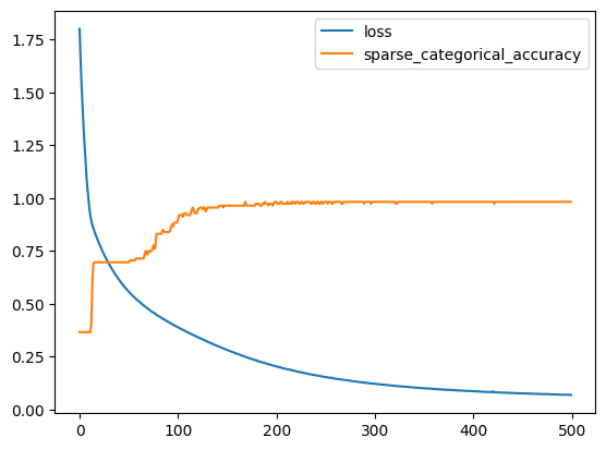
2,整体准确率

test_loss, test_acc = model.evaluate(X_test, y_test, verbose=2)
print(' %.2f%%' %(test_acc*100))

2/2 - 0s - loss: 0.1298 - sparse_categorical_accuracy: 0.9737 - 271ms/epoch - 135ms/step
 97.37%

3,预测样本

predictions = model.predict(X_test, verbose=2)
print(predictions[0])
print(' %d %.2f%%' %(tf.argmax(predictions[0]), max(predictions[0])*100))

2/2 - 0s - 104ms/epoch - 52ms/step
[8.3498879e-09 1.8262751e-03 9.9817371e-01]
 2 99.82%

print(predictions)

[[8.3498879e-09 1.8262751e-03 9.9817371e-01]
 [3.2518408e-03 9.8306483e-01 1.3683353e-02]
 [9.9939382e-01 6.0616154e-04 4.0472346e-14]
 [5.1105918e-08 1.5814977e-02 9.8418498e-01]
 [9.9613428e-01 3.8657226e-03 1.1263443e-11]
 [5.0845561e-10 4.7897341e-04 9.9952102e-01]
 [9.9715734e-01 2.8426135e-03 4.8997234e-12]
 [7.0876861e-04 9.6024650e-01 3.9044708e-02]
 [4.2222903e-04 9.3484229e-01 6.4735457e-02]
 [4.0413835e-03 9.8746198e-01 8.4966142e-03]
 [1.2660873e-06 4.3164853e-02 9.5683390e-01]
 [1.3402370e-03 9.7123307e-01 2.7426608e-02]
 [8.4431336e-04 9.0923429e-01 8.9921355e-02]
 [4.3927005e-04 9.0233898e-01 9.7221702e-02]
 [4.7115324e-04 8.2901543e-01 1.7051351e-01]
 [9.9828017e-01 1.7199020e-03 1.7988909e-12]
 [5.4972956e-04 8.3909136e-01 1.6035888e-01]
 [8.9530699e-04 8.0865324e-01 1.9045144e-01]
 [9.9046409e-01 9.5359245e-03 1.5190581e-10]
 [9.9846578e-01 1.5342035e-03 4.7513046e-13]
 [5.6102238e-07 1.9395353e-02 9.8060405e-01]
 [5.0135364e-04 7.1416974e-01 2.8532892e-01]
 [9.9001676e-01 9.9832211e-03 2.1078256e-10]
 [9.9051952e-01 9.4804186e-03 3.4175113e-10]
 [2.6071793e-05 2.8323361e-01 7.1674031e-01]
 [9.9886900e-01 1.1309125e-03 1.0174007e-12]
 [9.9197525e-01 8.0247913e-03 6.7378651e-11]
 [2.3211068e-03 9.8043609e-01 1.7242851e-02]
 [1.7626515e-02 9.7543079e-01 6.9427858e-03]
 [9.9145693e-01 8.5430704e-03 8.4697659e-11]
 [2.2322536e-06 7.6802179e-02 9.2319554e-01]
 [3.9311437e-04 5.9891444e-01 4.0069246e-01]
 [9.9688905e-01 3.1109049e-03 4.3471437e-12]
 [2.7264292e-05 2.6483223e-01 7.3514050e-01]
 [8.7741050e-09 2.8957480e-03 9.9710423e-01]
 [2.0027638e-03 8.8426864e-01 1.1372862e-01]
 [9.9712950e-01 2.8704719e-03 1.3951041e-12]
 [7.7986178e-06 1.2152320e-01 8.7846905e-01]]

4,输出混淆矩阵

from sklearn.metrics import confusion_matrix, classification_report
y_true = y_test
y_pred = np.argmax(predictions, axis=1)
print(confusion_matrix(y_true, y_pred))

[[13  0  0]
 [ 0 15  1]
 [ 0  0  9]]

分类报告

print(classification_report(y_true, y_pred))

              precision    recall  f1-score   support

           0       1.00      1.00      1.00        13
           1       1.00      0.94      0.97        16
           2       0.90      1.00      0.95         9

    accuracy                           0.97        38
   macro avg       0.97      0.98      0.97        38
weighted avg       0.98      0.97      0.97        38

模型结构

print(model.summary())

Model: "sequential"
_________________________________________________________________
 Layer (type)                Output Shape              Param #   
=================================================================
 dense (Dense)               (None, 10)                50        

 dense_1 (Dense)             (None, 3)                 33        

=================================================================
Total params: 83
Trainable params: 83
Non-trainable params: 0
_________________________________________________________________
None

用tensorflow实现fashion-mnist服饰分类

import numpy as np
import pandas as pd
import matplotlib.pyplot as plt
import tensorflow as tf

①导数据集

(x_train, y_train), (x_test, y_test) = tf.keras.datasets.fashion_mnist.load_data()

Downloading data from https://storage.googleapis.com/tensorflow/tf-keras-datasets/train-labels-idx1-ubyte.gz
29515/29515 [==============================] - 0s 6us/step
Downloading data from https://storage.googleapis.com/tensorflow/tf-keras-datasets/train-images-idx3-ubyte.gz
26421880/26421880 [==============================] - 18s 1us/step
Downloading data from https://storage.googleapis.com/tensorflow/tf-keras-datasets/t10k-labels-idx1-ubyte.gz
5148/5148 [==============================] - 0s 0s/step
Downloading data from https://storage.googleapis.com/tensorflow/tf-keras-datasets/t10k-images-idx3-ubyte.gz
4422102/4422102 [==============================] - 4s 1us/step

②探索数据

1,基本描述信息

print( "x_train shape:", x_train.shape, "y_train shape:", y_train.shape)
print( "x_test shape:", x_test.shape, "y_test shape:", y_test.shape)
print(y_train[:20]) #前20个label
print(len(x_train)) #训练集样本个数

x_train shape: (60000, 28, 28) y_train shape: (60000,)
x_test shape: (10000, 28, 28) y_test shape: (10000,)
[9 0 0 3 0 2 7 2 5 5 0 9 5 5 7 9 1 0 6 4]
60000

2,显示单张图片

plt.imshow(x_train[0], cmap = 'gray')
plt.colorbar()
plt.grid(False)
plt.show()

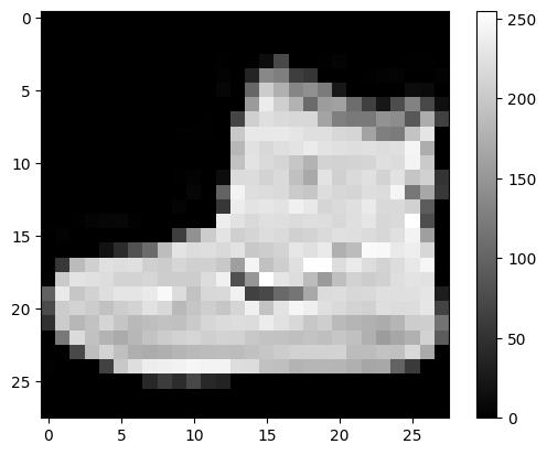
3,显示多张图片

class_names = ['T-shirt', 'Trouser', 'Pullover', 'Dress', 'Coat', 'Sandal', 'Shirt', 'Sneaker', 'Bag', 'Ankle boot']
plt.figure(figsize=(10,10))
for i in range(25):
    plt.subplot(5,5,i+1)
    plt.xticks([])
    plt.yticks([])
    plt.grid(False)
    plt.imshow(x_train[i], cmap=plt.cm.binary)
    plt.xlabel(class_names[y_train[i]])
plt.show()

4,标准化

x_train = x_train / 255.0
x_test = x_test / 255.0

③构建模型

1,定义层

model = tf.keras.models.Sequential([tf.keras.layers.Flatten(input_shape = (28, 28)),
 tf.keras.layers.Dense(128, activation ='relu'),
 tf.keras.layers.Dropout(0.05),
 tf.keras.layers.Dense(10, activation ='softmax')
])

2,编译模型

model.compile(optimizer='adam',
 loss=tf.keras.losses.SparseCategoricalCrossentropy(from_logits=False),
 metrics=['accuracy'])

3,查看模型结构

model.summary()

Model: "sequential_1"
_________________________________________________________________
 Layer (type)                Output Shape              Param #   
=================================================================
 flatten (Flatten)           (None, 784)               0         

 dense_2 (Dense)             (None, 128)               100480    

 dropout (Dropout)           (None, 128)               0         

 dense_3 (Dense)             (None, 10)                1290      

=================================================================
Total params: 101,770
Trainable params: 101,770
Non-trainable params: 0
_________________________________________________________________

④训练模型

1,训练集训练,迭代10次

history = model.fit(x_train, y_train, epochs=10)

Epoch 1/10
1875/1875 [==============================] - 6s 3ms/step - loss: 0.5066 - accuracy: 0.8221
Epoch 2/10
1875/1875 [==============================] - 4s 2ms/step - loss: 0.3800 - accuracy: 0.8615
Epoch 3/10
1875/1875 [==============================] - 4s 2ms/step - loss: 0.3409 - accuracy: 0.8751
Epoch 4/10
1875/1875 [==============================] - 4s 2ms/step - loss: 0.3187 - accuracy: 0.8837
Epoch 5/10
1875/1875 [==============================] - 4s 2ms/step - loss: 0.3024 - accuracy: 0.8886
Epoch 6/10
1875/1875 [==============================] - 3s 2ms/step - loss: 0.2891 - accuracy: 0.8931
Epoch 7/10
1875/1875 [==============================] - 4s 2ms/step - loss: 0.2781 - accuracy: 0.8962
Epoch 8/10
1875/1875 [==============================] - 3s 2ms/step - loss: 0.2672 - accuracy: 0.9004
Epoch 9/10
1875/1875 [==============================] - 4s 2ms/step - loss: 0.2577 - accuracy: 0.9037
Epoch 10/10
1875/1875 [==============================] - 4s 2ms/step - loss: 0.2508 - accuracy: 0.9056

显示每个epoch loss和accuracy的历史值

history.history

{'loss': [0.506623387336731,
  0.37999778985977173,
  0.3408657908439636,
  0.3187374770641327,
  0.3024260997772217,
  0.2890622913837433,
  0.27812787890434265,
  0.26724332571029663,
  0.2576807737350464,
  0.25076183676719666],
 'accuracy': [0.8220666646957397,
  0.8614500164985657,
  0.8751000165939331,
  0.8837000131607056,
  0.888616681098938,
  0.8930500149726868,
  0.8961833119392395,
  0.9004499912261963,
  0.9036833047866821,
  0.9056166410446167]}

图形化训练过程

def plot_learning_curves(history):
    pd.DataFrame(history.history).plot(figsize = (8, 5))
    plt.grid(True)
    plt.gca().set_ylim(0,1)
    plt.show()
plot_learning_curves(history)

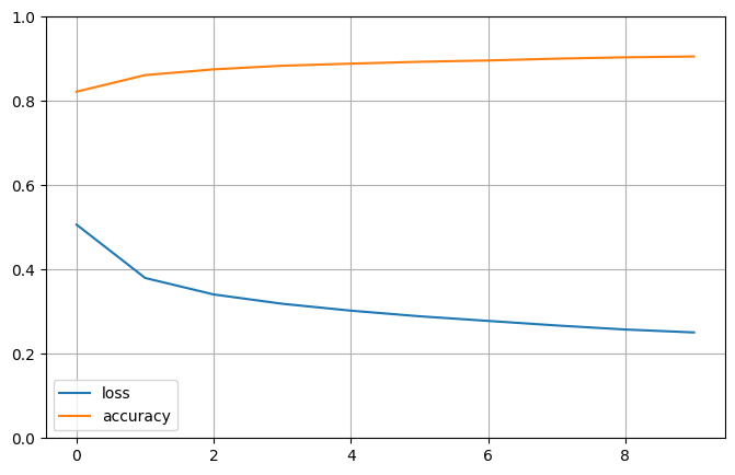
2,用测试集评估准确率

test_loss, test_acc = model.evaluate(x_test, y_test, verbose=2) 
print('\nTest accuracy:', test_acc) 
predictions = model.predict(x_test) 
print(predictions[0]) 
print(' %d , %.2f%%' %(np.argmax(predictions[0]), max((predictions[0]))*100)) 

313/313 - 1s - loss: 0.3281 - accuracy: 0.8826 - 1s/epoch - 4ms/step

Test accuracy: 0.8826000094413757
313/313 [==============================] - 1s 2ms/step
[2.8944891e-07 9.0106245e-10 3.1913419e-08 1.7882961e-09 3.8579850e-07
 4.8054244e-02 1.7083392e-08 1.9777216e-01 1.4086240e-06 7.5417143e-01]
 9 , 75.42%

用卷积神经网络实现fashion-mnist服饰分类

import matplotlib.pyplot as plt
import numpy as np
import pandas as pd
import tensorflow as tf
from tensorflow import keras
from sklearn.metrics import confusion_matrix, classification_report
import os

①读取数据,理解图像

(x_train, y_train), (x_test, y_test) = tf.keras.datasets.fashion_mnist.load_data() 
x_train = x_train.reshape(-1, 28, 28, 1).astype('float32')
x_test = x_test.reshape(-1, 28, 28, 1).astype('float32') 
input_shape = (28, 28, 1)

②标准化

x_train = x_train / 255.0
x_test = x_test / 255.0

③搭建模型

1,第一个卷积层

model = keras.models.Sequential() 
model.add(keras.layers.Conv2D(filters=128, kernel_size=(3,3), input_shape=input_shape))
model.add(keras.layers.BatchNormalization()) 
model.add(keras.layers.Activation('relu'))
model.add(keras.layers.MaxPool2D(pool_size=(2,2), strides=2))

2,第二个卷积层

model.add(keras.layers.Conv2D(filters=64, kernel_size=(3,3)))
model.add(keras.layers.BatchNormalization())
model.add(keras.layers.Activation('relu')) 
model.add(keras.layers.MaxPool2D(pool_size=(2,2), strides=2))
model.add(keras.layers.Dropout(0.2)) 

3,全连接层

model.add(keras.layers.Flatten())
model.add(keras.layers.Dense(128, activation = 'relu'))
model.add(keras.layers.Dropout(0.2))
model.add(keras.layers.Dense(64, activation = 'relu')) 
model.add(keras.layers.Dropout(0.2)) #
model.add(keras.layers.Dense(10, activation = 'softmax')) 

④编译模型

model.compile(loss = 'sparse_categorical_crossentropy', optimizer = 'adam', metrics =['sparse_categorical_accuracy'])
model.summary()

Model: "sequential_2"
_________________________________________________________________
 Layer (type)                Output Shape              Param #   
=================================================================
 conv2d (Conv2D)             (None, 26, 26, 128)       1280      

 batch_normalization (BatchN  (None, 26, 26, 128)      512       
 ormalization)                                                   

 activation (Activation)     (None, 26, 26, 128)       0         

 max_pooling2d (MaxPooling2D  (None, 13, 13, 128)      0         
 )                                                               

 conv2d_1 (Conv2D)           (None, 11, 11, 64)        73792     

 batch_normalization_1 (Batc  (None, 11, 11, 64)       256       
 hNormalization)                                                 

 activation_1 (Activation)   (None, 11, 11, 64)        0         

 max_pooling2d_1 (MaxPooling  (None, 5, 5, 64)         0         
 2D)                                                             

 dropout_1 (Dropout)         (None, 5, 5, 64)          0         

 flatten_1 (Flatten)         (None, 1600)              0         

 dense_4 (Dense)             (None, 128)               204928    

 dropout_2 (Dropout)         (None, 128)               0         

 dense_5 (Dense)             (None, 64)                8256      

 dropout_3 (Dropout)         (None, 64)                0         

 dense_6 (Dense)             (None, 10)                650       

=================================================================
Total params: 289,674
Trainable params: 289,290
Non-trainable params: 384
_________________________________________________________________

⑤训练

1,断点续训

checkpoint_save_path = 'checkpoint_CNN/mnist.ckpt'
if os.path.exists(checkpoint_save_path + '.index'):
    print('----------load the model----------')
    model.load_weights(checkpoint_save_path)
cp_callback = tf.keras.callbacks.ModelCheckpoint(filepath=checkpoint_save_path, save_weights_only=True,
save_best_only=True)

2,训练

迭代30次,一次需要80s,进40mins

history = model.fit(x_train, y_train, epochs = 30, validation_data = (x_test, y_test),
callbacks=[cp_callback]) 

Epoch 1/30
1875/1875 [==============================] - 84s 44ms/step - loss: 0.5458 - sparse_categorical_accuracy: 0.8037 - val_loss: 0.4283 - val_sparse_categorical_accuracy: 0.8342
Epoch 2/30
1875/1875 [==============================] - 83s 44ms/step - loss: 0.3664 - sparse_categorical_accuracy: 0.8682 - val_loss: 0.3810 - val_sparse_categorical_accuracy: 0.8411
Epoch 3/30
1875/1875 [==============================] - 87s 47ms/step - loss: 0.3224 - sparse_categorical_accuracy: 0.8842 - val_loss: 0.2943 - val_sparse_categorical_accuracy: 0.8939
Epoch 4/30
1875/1875 [==============================] - 85s 45ms/step - loss: 0.2976 - sparse_categorical_accuracy: 0.8929 - val_loss: 0.3043 - val_sparse_categorical_accuracy: 0.8864
Epoch 5/30
1875/1875 [==============================] - 87s 46ms/step - loss: 0.2754 - sparse_categorical_accuracy: 0.8986 - val_loss: 0.2799 - val_sparse_categorical_accuracy: 0.8988
Epoch 6/30
1875/1875 [==============================] - 77s 41ms/step - loss: 0.2570 - sparse_categorical_accuracy: 0.9059 - val_loss: 0.2563 - val_sparse_categorical_accuracy: 0.9066
Epoch 7/30
1875/1875 [==============================] - 79s 42ms/step - loss: 0.2430 - sparse_categorical_accuracy: 0.9106 - val_loss: 0.2726 - val_sparse_categorical_accuracy: 0.9034
Epoch 8/30
1875/1875 [==============================] - 87s 46ms/step - loss: 0.2316 - sparse_categorical_accuracy: 0.9151 - val_loss: 0.2493 - val_sparse_categorical_accuracy: 0.9125
Epoch 9/30
1875/1875 [==============================] - 85s 45ms/step - loss: 0.2187 - sparse_categorical_accuracy: 0.9195 - val_loss: 0.2665 - val_sparse_categorical_accuracy: 0.9034
Epoch 10/30
1875/1875 [==============================] - 77s 41ms/step - loss: 0.2126 - sparse_categorical_accuracy: 0.9221 - val_loss: 0.2390 - val_sparse_categorical_accuracy: 0.9137
Epoch 11/30
1875/1875 [==============================] - 81s 43ms/step - loss: 0.2038 - sparse_categorical_accuracy: 0.9250 - val_loss: 0.2509 - val_sparse_categorical_accuracy: 0.9136
Epoch 12/30
1875/1875 [==============================] - 78s 42ms/step - loss: 0.1945 - sparse_categorical_accuracy: 0.9277 - val_loss: 0.2683 - val_sparse_categorical_accuracy: 0.9055
Epoch 13/30
1875/1875 [==============================] - 78s 42ms/step - loss: 0.1883 - sparse_categorical_accuracy: 0.9289 - val_loss: 0.2644 - val_sparse_categorical_accuracy: 0.9032
Epoch 14/30
1875/1875 [==============================] - 79s 42ms/step - loss: 0.1838 - sparse_categorical_accuracy: 0.9315 - val_loss: 0.2439 - val_sparse_categorical_accuracy: 0.9133
Epoch 15/30
1875/1875 [==============================] - 78s 42ms/step - loss: 0.1743 - sparse_categorical_accuracy: 0.9349 - val_loss: 0.2571 - val_sparse_categorical_accuracy: 0.9130
Epoch 16/30
1875/1875 [==============================] - 79s 42ms/step - loss: 0.1710 - sparse_categorical_accuracy: 0.9359 - val_loss: 0.2388 - val_sparse_categorical_accuracy: 0.9177
Epoch 17/30
1875/1875 [==============================] - 78s 42ms/step - loss: 0.1683 - sparse_categorical_accuracy: 0.9381 - val_loss: 0.2838 - val_sparse_categorical_accuracy: 0.9087
Epoch 18/30
1875/1875 [==============================] - 78s 42ms/step - loss: 0.1604 - sparse_categorical_accuracy: 0.9409 - val_loss: 0.2425 - val_sparse_categorical_accuracy: 0.9172
Epoch 19/30
1875/1875 [==============================] - 80s 43ms/step - loss: 0.1576 - sparse_categorical_accuracy: 0.9401 - val_loss: 0.2568 - val_sparse_categorical_accuracy: 0.9161
Epoch 20/30
1875/1875 [==============================] - 84s 45ms/step - loss: 0.1572 - sparse_categorical_accuracy: 0.9409 - val_loss: 0.2672 - val_sparse_categorical_accuracy: 0.9076
Epoch 21/30
1875/1875 [==============================] - 82s 44ms/step - loss: 0.1506 - sparse_categorical_accuracy: 0.9434 - val_loss: 0.2643 - val_sparse_categorical_accuracy: 0.9124
Epoch 22/30
1875/1875 [==============================] - 82s 44ms/step - loss: 0.1496 - sparse_categorical_accuracy: 0.9449 - val_loss: 0.2574 - val_sparse_categorical_accuracy: 0.9160
Epoch 23/30
1875/1875 [==============================] - 79s 42ms/step - loss: 0.1448 - sparse_categorical_accuracy: 0.9457 - val_loss: 0.2454 - val_sparse_categorical_accuracy: 0.9162
Epoch 24/30
1875/1875 [==============================] - 79s 42ms/step - loss: 0.1396 - sparse_categorical_accuracy: 0.9473 - val_loss: 0.2552 - val_sparse_categorical_accuracy: 0.9171
Epoch 25/30
1875/1875 [==============================] - 81s 43ms/step - loss: 0.1417 - sparse_categorical_accuracy: 0.9478 - val_loss: 0.2597 - val_sparse_categorical_accuracy: 0.9180
Epoch 26/30
1875/1875 [==============================] - 82s 44ms/step - loss: 0.1379 - sparse_categorical_accuracy: 0.9479 - val_loss: 0.2551 - val_sparse_categorical_accuracy: 0.9192
Epoch 27/30
1875/1875 [==============================] - 81s 43ms/step - loss: 0.1347 - sparse_categorical_accuracy: 0.9493 - val_loss: 0.3071 - val_sparse_categorical_accuracy: 0.8981
Epoch 28/30
1875/1875 [==============================] - 81s 43ms/step - loss: 0.1282 - sparse_categorical_accuracy: 0.9520 - val_loss: 0.2555 - val_sparse_categorical_accuracy: 0.9149
Epoch 29/30
1875/1875 [==============================] - 81s 43ms/step - loss: 0.1286 - sparse_categorical_accuracy: 0.9523 - val_loss: 0.2935 - val_sparse_categorical_accuracy: 0.9121
Epoch 30/30
1875/1875 [==============================] - 82s 44ms/step - loss: 0.1264 - sparse_categorical_accuracy: 0.9542 - val_loss: 0.2639 - val_sparse_categorical_accuracy: 0.9153

3,绘制acc和loss曲线

def plot_learning_curves(history):
    pd.DataFrame(history.history).plot(figsize=(8,5))
    plt.grid(True)
    plt.ylim(0, 1)
    plt.show()
plot_learning_curves(history)

4,保存模型

model.save('fashion_model.h5')

⑥评估和预测

1,评估evaluate

test_loss, test_acc = model.evaluate(x_test, y_test, verbose=2)
print('\nTest accuracy:', test_acc)

313/313 - 4s - loss: 0.2639 - sparse_categorical_accuracy: 0.9153 - 4s/epoch - 12ms/step

Test accuracy: 0.9153000116348267

2,预测predict

predictions = model.predict(x_test)
print(predictions[0])
print(' %d , %.2f%%' %(np.argmax(predictions[0]), max((predictions[0]))*100))

313/313 [==============================] - 4s 12ms/step
[1.9348605e-17 2.0841505e-16 7.7804646e-13 1.9641095e-16 8.0456529e-13
 1.6399678e-08 3.9137113e-13 1.6209668e-06 2.5761291e-14 9.9999833e-01]
 9 , 100.00%

⑦查看模型分类效果

1,绘制混淆矩阵

y_true = y_test
y_pred = np.argmax(predictions, axis=1)
pd.crosstab(y_true, y_pred)
confusion_matrix(y_true, y_pred)

array([[800,   1,  18,  27,   1,   0, 145,   0,   8,   0],
       [  1, 982,   0,  10,   1,   0,   3,   0,   3,   0],
       [ 13,   0, 850,   7,  53,   0,  76,   0,   1,   0],
       [  9,   3,  13, 929,  16,   0,  29,   0,   1,   0],
       [  0,   0,  33,  18, 868,   0,  80,   0,   1,   0],
       [  0,   0,   0,   0,   0, 980,   0,  13,   0,   7],
       [ 57,   2,  44,  27,  44,   0, 819,   0,   7,   0],
       [  0,   0,   0,   0,   0,   6,   0, 981,   0,  13],
       [  1,   0,   2,   3,   0,   1,   5,   1, 987,   0],
       [  0,   0,   0,   0,   0,   5,   0,  38,   0, 957]], dtype=int64)

2,打印分类报告

print(classification_report(y_true, y_pred))

              precision    recall  f1-score   support

           0       0.91      0.80      0.85      1000
           1       0.99      0.98      0.99      1000
           2       0.89      0.85      0.87      1000
           3       0.91      0.93      0.92      1000
           4       0.88      0.87      0.88      1000
           5       0.99      0.98      0.98      1000
           6       0.71      0.82      0.76      1000
           7       0.95      0.98      0.97      1000
           8       0.98      0.99      0.98      1000
           9       0.98      0.96      0.97      1000

    accuracy                           0.92     10000
   macro avg       0.92      0.92      0.92     10000
weighted avg       0.92      0.92      0.92     10000