深度学习——LeNet卷积神经网络初探

LeNet--卷积神经网络初探

模型介绍：

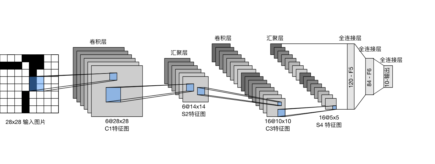
简单介绍： 从网络结构可以看出LeNet对于现在的大模型来说是一个非常小的神经网络，他一共由7个层顺序连接组成。分别是卷积层、pooling层、卷积层、pooling层和三个全连接层。用现代的深度学习框架来实现代码如下：

代码实现和解读：

net = nn.Sequential(
    nn.Conv2d(1, 6, kernel_size=5, padding=2), nn.Sigmoid(),
    nn.AvgPool2d(kernel_size=2, stride=2),
    nn.Conv2d(6, 16, kernel_size=5), nn.Sigmoid(),
    nn.AvgPool2d(kernel_size=2, stride=2), nn.Flatten(),
    nn.Linear(16 * 5 * 5, 120), nn.Sigmoid(),
    nn.Linear(120, 84), nn.Sigmoid(),
    nn.Linear(84, 10))

解读： 这一部分是有关网络的定义，可以看出网络的基本层实现都调用了torch的库，sigmoid() 函数的作用是：让网络中各层叠加后不会坍缩，因为引入了非线性函数。我们来输出一下网络的各层的结构。

X = torch.rand(size=(1, 1, 28, 28), dtype=torch.float32)

for layer in net:
    X = layer(X)
    print(layer.__class__.__name__, 'output shape: \t:', X.shape)

Conv2d output shape: 	: torch.Size([1, 6, 28, 28])
Sigmoid output shape: 	: torch.Size([1, 6, 28, 28])
AvgPool2d output shape: : torch.Size([1, 6, 14, 14])
Conv2d output shape: 	: torch.Size([1, 16, 10, 10])
Sigmoid output shape: 	: torch.Size([1, 16, 10, 10])
AvgPool2d output shape: : torch.Size([1, 16, 5, 5])
Flatten output shape: 	: torch.Size([1, 400])
Linear output shape: 	: torch.Size([1, 120])
Sigmoid output shape: 	: torch.Size([1, 120])
Linear output shape: 	: torch.Size([1, 84])
Sigmoid output shape: 	: torch.Size([1, 84])
Linear output shape: 	: torch.Size([1, 10])

接下来我们利用沐神的d2l包中的数据集准备函数来下载MNIST数据集。

def evaluate_accuracy_gpu(net, data_iter, device=None):
    if isinstance(net, nn.Module):  # * 判断变量的类型
        net.eval()          
        #? 将网络设置为评估模式, 在此模式下，net会关闭一些特定的训练技巧以确保网络的行为和训练时一致
        if not device:
            device = next(iter(net.parameters())).device
    metric = d2l.Accumulator(2)
    with torch.no_grad():
        for X, y in data_iter:
            if isinstance(X, list):
                X = [x.to(device) for x in X]
            else:
                X = X.to(device)  # * .to(device)是为了将数据送至指定的设备上进行计算
            y = y.to(device)
            metric.add(d2l.accuracy(net(X), y), y.numel())
    return metric[0] / metric[1]  # * 这里返回的是预测精度

以上的这段代码的关键步骤是执行了.to(device)操作，上述方法作用的调用可用的GPU进行加速运算。

接下来这段代码是对net执行训练的方法定义：

def train_ch6(net, train_iter, test_iter, num_epochs, lr, device):
    def init_weights(m):
        if type(m) == nn.Linear or type(m) == nn.Conv2d:
            nn.init.xavier_uniform_(m.weight)  # ? 初始化参数
            
    net.apply(init_weights)
    print('training on', device)
    net.to(device)
    optimizer = torch.optim.SGD(net.parameters(), lr=lr)
    loss = nn.CrossEntropyLoss()  # ? 交叉熵损失函数
    animator = d2l.Animator(xlabel='epoch', xlim=[3, num_epochs], ylim=[0, 2],legend=['train loss', 'train acc', 'test acc'])
    timer, num_batches = d2l.Timer(), len(train_iter)
    for epoch in range(num_epochs):
        metric = d2l.Accumulator(3)
        net.train()  # ? 将网络设置为训练模式
        for i, (X, y) in enumerate(train_iter):  # ? enumerate会返回索引同时返回对应迭代次数时的元素
            optimizer.zero_grad()
            X, y = X.to(device), y.to(device)
            y_hat = net(X)
            l = loss(y_hat, y)
            l.backward()
            optimizer.step()
            with torch.no_grad():
                metric.add(l * X.shape[0], d2l.accuracy(y_hat, y), X.shape[0])
            timer.stop()
            train_l = metric[0] / metric[1]
            train_acc = metric[1] / metric[2]
            if (i + 1) % (num_batches // 5) == 0 or i == num_batches - 1:
                animator.add(epoch + (i + 1) / num_batches, (train_l, train_acc, None))
        test_acc = evaluate_accuracy_gpu(net, test_iter)
        animator.add(epoch + 1, (None, None, test_acc))
    print(f'loss {train_l:.3f}, train acc {train_acc:.3f}, ' f'test acc {test_acc:.3f}')
    print(f'{metric[2]*num_epochs / timer.sum():.1f} examples/sec ' f'on {str(device)}')

这段代码非常的长，我们将其分为几个部分来进行解读：

首先：

def init_weights(m):
    if type(m) == nn.Linear or type(m) == nn.Conv2d:
        nn.init.xavier_uniform_(m.weight)  # ? 初始化参数
            
    net.apply(init_weights)

这一段摘要做的是网络所有参数的初始化。

其次：

print('training on', device)
net.to(device)
optimizer = torch.optim.SGD(net.parameters(), lr=lr)
loss = nn.CrossEntropyLoss()  # ? 交叉熵损失函数
animator = d2l.Animator(xlabel='epoch', xlim=[3, num_epochs], ylim=[0, 2],legend=['train loss', 'train acc', 'test acc'])
timer, num_batches = d2l.Timer(), len(train_iter)

这一段主要是定义了网络训练和结果可视化的必要变量，并将网络放在GPU上进行运行。

接下来：

for epoch in range(num_epochs):
    metric = d2l.Accumulator(3)
    net.train()  # ? 将网络设置为训练模式
    for i, (X, y) in enumerate(train_iter):  # ? enumerate会返回索引同时返回对应迭代次数时的元素
        optimizer.zero_grad()
        X, y = X.to(device), y.to(device)
        y_hat = net(X)
        l = loss(y_hat, y)
        l.backward()
        optimizer.step()
        with torch.no_grad():
            metric.add(l * X.shape[0], d2l.accuracy(y_hat, y), X.shape[0])
        timer.stop()
        train_l = metric[0] / metric[1]
        train_acc = metric[1] / metric[2]
        if (i + 1) % (num_batches // 5) == 0 or i == num_batches - 1:
            animator.add(epoch + (i + 1) / num_batches, (train_l, train_acc, None))
    test_acc = evaluate_accuracy_gpu(net, test_iter)
    animator.add(epoch + 1, (None, None, test_acc))

这一部分是最重要的训练部分：前向传导、计算损失、对损失进行反向传导并计算梯度、根据梯度来更新参数。对每一个样本都进行上述的基本过程。

剩下的部分就是对训练的中间过程进行适当的输出。

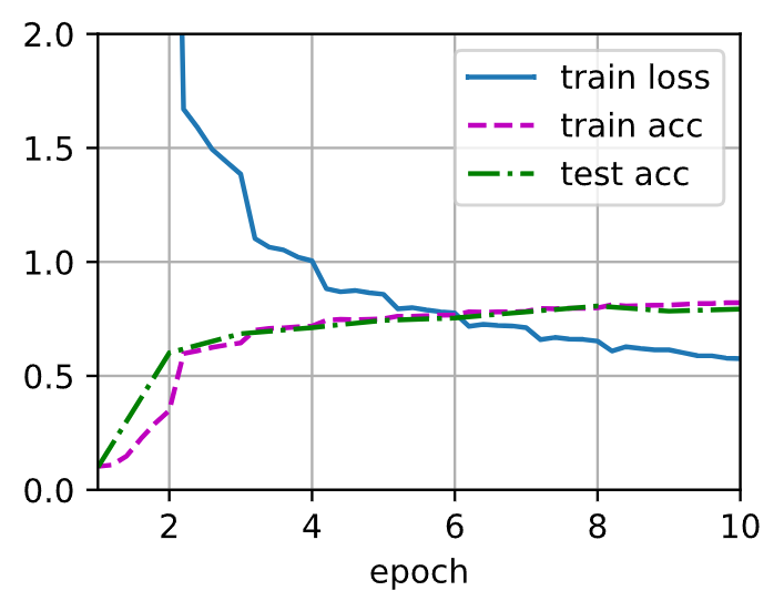
lr, num_epochs = 0.9, 10
train_ch6(net, train_iter, test_iter, num_epochs, lr, d2l.try_gpu())

这段代码描述的是网络训练器使用的过程。根据上述参数定义，得到的训练结果如下图：

模型局部最优化：

接下来，我想做的是，利用循环和结果可视化来找到这个模型下的局部最优超参数。