Python数据分析与机器学习-逻辑回归案例分析
Logistic Regression
The Data
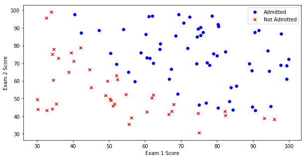
我们将建立一个逻辑回归模型来预测一个学生是否被大学录取。假设你是一个大学系的管理员,你想根据两次考试的结果来决定每个申请人的录取机会。你有以前的申请人的历史数据,你可以用它作为逻辑回归的训练集。对于每一个培训例子,你有两个考试的申请人的分数和录取决定。为了做到这一点,我们将建立一个分类模型,根据考试成绩估计入学概率。
# 三大件
import numpy as np
import pandas as pd
import matplotlib.pyplot as plt
%matplotlib inline
import os
path = 'data'+os.sep+'LogiReg_data.txt'
pdData = pd.read_csv(path,header=None,names=['Exam 1','Exam 2','Admitted'])
pdData.head()
| Exam 1 | Exam 2 | Admitted | |
|---|---|---|---|
| 0 | 34.623660 | 78.024693 | 0 |
| 1 | 30.286711 | 43.894998 | 0 |
| 2 | 35.847409 | 72.902198 | 0 |
| 3 | 60.182599 | 86.308552 | 1 |
| 4 | 79.032736 | 75.344376 | 1 |
pdData.shape
(100, 3)
positive = pdData[pdData['Admitted']==1]
negative = pdData[pdData['Admitted']==0]
negative.head()

fig,ax = plt.subplots(figsize=(10,5))
ax.scatter(positive['Exam 1'],positive['Exam 2'],s=30,c='b',marker='o',label='Admitted')
ax.scatter(negative['Exam 1'],negative['Exam 2'],s=30,c='r',marker='x',label='Not Admitted')
ax.legend()
ax.set_xlabel('Exam 1 Score')
ax.set_ylabel('Exam 2 Score')
Text(0, 0.5, 'Exam 2 Score')
The logistic regression
目标:建立分类器(求解出三个参数\(\theta_0,\theta_1,\theta_2\))
设定阈值,根据阈值判断录取结果
要完成的模块
sigmoid:映射到概率的函数model:返回预测结果值cost:根据参数计算损失gradient:计算每个参数的梯度方向descent:进行参数更新accuracy:计算精度
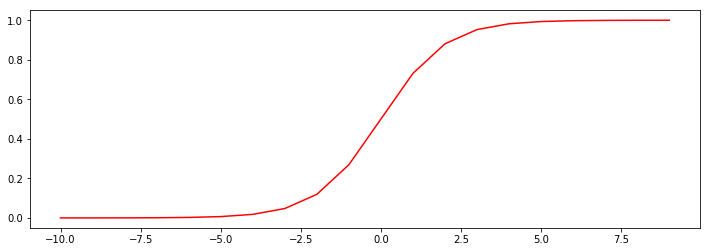
Sigmoid 函数
\[g(z) = \frac{1}{1+e^{-z}}
\]
- \(g:\mathbb{R} \to [0,1]\)
- \(g(0)=0.5\)
- \(g(- \infty)=0\)
- \(g(+ \infty)=1\)
def sigmoid(z):
    return 1/(1+np.exp(-z))
nums = np.arange(-10,10,step=1)
print(nums)
fig,ax = plt.subplots(figsize=(12,4))
ax.plot(nums,sigmoid(nums),'r')
plt.show()
[-10  -9  -8  -7  -6  -5  -4  -3  -2  -1   0   1   2   3   4   5   6   7
   8   9]
def model(X,theta):
    """ Returns our model result
    :param X: examples to classify, m x p
    :param theta: parameters,  p x 1
    :return: the sigmoid evaluated for each examples in X given parameters theta as a m x 1 vector
    """
    return sigmoid(np.matmul(X,theta))
\[\begin{array}{ccc}
\begin{pmatrix} 1 & x_{1} & x_{2}\end{pmatrix} & \times & \begin{pmatrix}\theta_{0}\\
\theta_{1}\\
\theta_{2}
\end{pmatrix}\end{array}=\theta_{0}+\theta_{1}x_{1}+\theta_{2}x_{2}
\]
pdData.insert(0,'Ones',1)
pdData.head()

# set X (training data) and y (target variable)
orig_data = pdData.as_matrix() # convert the Pandas representation of the data to an array useful for further computations
print(orig_data)
cols = orig_data.shape[1]
print(cols)
X = orig_data[:,0:cols-1]
y = orig_data[:,cols-1:cols]

# print(X[:5])
theta = np.zeros([cols-1,1])
[[ 1.         34.62365962 78.02469282  0.        ]
 [ 1.         30.28671077 43.89499752  0.        ]
 [ 1.         35.84740877 72.90219803  0.        ]
 [ 1.         60.18259939 86.3085521   1.        ]
 [ 1.         79.03273605 75.34437644  1.        ]
 [ 1.         45.08327748 56.31637178  0.        ]
 [ 1.         61.10666454 96.51142588  1.        ]
 [ 1.         75.02474557 46.55401354  1.        ]
 [ 1.         76.0987867  87.42056972  1.        ]
 [ 1.         84.43281996 43.53339331  1.        ]
 [ 1.         95.86155507 38.22527806  0.        ]
 [ 1.         75.01365839 30.60326323  0.        ]
 [ 1.         82.30705337 76.4819633   1.        ]
 [ 1.         69.36458876 97.71869196  1.        ]
 [ 1.         39.53833914 76.03681085  0.        ]
 [ 1.         53.97105215 89.20735014  1.        ]
 [ 1.         69.07014406 52.74046973  1.        ]
 [ 1.         67.94685548 46.67857411  0.        ]
 [ 1.         70.66150955 92.92713789  1.        ]
 [ 1.         76.97878373 47.57596365  1.        ]
 [ 1.         67.37202755 42.83843832  0.        ]
 [ 1.         89.67677575 65.79936593  1.        ]
 [ 1.         50.53478829 48.85581153  0.        ]
 [ 1.         34.21206098 44.2095286   0.        ]
 [ 1.         77.92409145 68.97235999  1.        ]
 [ 1.         62.27101367 69.95445795  1.        ]
 [ 1.         80.19018075 44.82162893  1.        ]
 [ 1.         93.1143888  38.80067034  0.        ]
 [ 1.         61.83020602 50.25610789  0.        ]
 [ 1.         38.7858038  64.99568096  0.        ]
 [ 1.         61.37928945 72.80788731  1.        ]
 [ 1.         85.40451939 57.05198398  1.        ]
 [ 1.         52.10797973 63.12762377  0.        ]
 [ 1.         52.04540477 69.43286012  1.        ]
 [ 1.         40.23689374 71.16774802  0.        ]
 [ 1.         54.63510555 52.21388588  0.        ]
 [ 1.         33.91550011 98.86943574  0.        ]
 [ 1.         64.17698887 80.90806059  1.        ]
 [ 1.         74.78925296 41.57341523  0.        ]
 [ 1.         34.18364003 75.23772034  0.        ]
 [ 1.         83.90239366 56.30804622  1.        ]
 [ 1.         51.54772027 46.85629026  0.        ]
 [ 1.         94.44336777 65.56892161  1.        ]
 [ 1.         82.36875376 40.61825516  0.        ]
 [ 1.         51.04775177 45.82270146  0.        ]
 [ 1.         62.22267576 52.06099195  0.        ]
 [ 1.         77.19303493 70.4582      1.        ]
 [ 1.         97.77159928 86.72782233  1.        ]
 [ 1.         62.0730638  96.76882412  1.        ]
 [ 1.         91.5649745  88.69629255  1.        ]
 [ 1.         79.94481794 74.16311935  1.        ]
 [ 1.         99.27252693 60.999031    1.        ]
 [ 1.         90.54671411 43.39060181  1.        ]
 [ 1.         34.52451385 60.39634246  0.        ]
 [ 1.         50.28649612 49.80453881  0.        ]
 [ 1.         49.58667722 59.80895099  0.        ]
 [ 1.         97.64563396 68.86157272  1.        ]
 [ 1.         32.57720017 95.59854761  0.        ]
 [ 1.         74.24869137 69.82457123  1.        ]
 [ 1.         71.79646206 78.45356225  1.        ]
 [ 1.         75.39561147 85.75993667  1.        ]
 [ 1.         35.28611282 47.02051395  0.        ]
 [ 1.         56.2538175  39.26147251  0.        ]
 [ 1.         30.05882245 49.59297387  0.        ]
 [ 1.         44.66826172 66.45008615  0.        ]
 [ 1.         66.56089447 41.09209808  0.        ]
 [ 1.         40.45755098 97.53518549  1.        ]
 [ 1.         49.07256322 51.88321182  0.        ]
 [ 1.         80.27957401 92.11606081  1.        ]
 [ 1.         66.74671857 60.99139403  1.        ]
 [ 1.         32.72283304 43.30717306  0.        ]
 [ 1.         64.03932042 78.03168802  1.        ]
 [ 1.         72.34649423 96.22759297  1.        ]
 [ 1.         60.45788574 73.0949981   1.        ]
 [ 1.         58.84095622 75.85844831  1.        ]
 [ 1.         99.8278578  72.36925193  1.        ]
 [ 1.         47.26426911 88.475865    1.        ]
 [ 1.         50.4581598  75.80985953  1.        ]
 [ 1.         60.45555629 42.50840944  0.        ]
 [ 1.         82.22666158 42.71987854  0.        ]
 [ 1.         88.91389642 69.8037889   1.        ]
 [ 1.         94.83450672 45.6943068   1.        ]
 [ 1.         67.31925747 66.58935318  1.        ]
 [ 1.         57.23870632 59.51428198  1.        ]
 [ 1.         80.366756   90.9601479   1.        ]
 [ 1.         68.46852179 85.5943071   1.        ]
 [ 1.         42.07545454 78.844786    0.        ]
 [ 1.         75.47770201 90.424539    1.        ]
 [ 1.         78.63542435 96.64742717  1.        ]
 [ 1.         52.34800399 60.76950526  0.        ]
 [ 1.         94.09433113 77.15910509  1.        ]
 [ 1.         90.44855097 87.50879176  1.        ]
 [ 1.         55.48216114 35.57070347  0.        ]
 [ 1.         74.49269242 84.84513685  1.        ]
 [ 1.         89.84580671 45.35828361  1.        ]
 [ 1.         83.48916274 48.3802858   1.        ]
 [ 1.         42.26170081 87.10385094  1.        ]
 [ 1.         99.31500881 68.77540947  1.        ]
 [ 1.         55.34001756 64.93193801  1.        ]
 [ 1.         74.775893   89.5298129   1.        ]]
4


C:\MyPrograms\Anaconda3\lib\site-packages\ipykernel_launcher.py:5: FutureWarning: Method .as_matrix will be removed in a future version. Use .values instead.
  """
X[:5]
array([[ 1.        , 34.62365962, 78.02469282],
       [ 1.        , 30.28671077, 43.89499752],
       [ 1.        , 35.84740877, 72.90219803],
       [ 1.        , 60.18259939, 86.3085521 ],
       [ 1.        , 79.03273605, 75.34437644]])
y[:5]
array([[0.],
       [0.],
       [0.],
       [1.],
       [1.]])
theta
array([[0.],
       [0.],
       [0.]])
X.shape,y.shape,theta.shape
((100, 3), (100, 1), (3, 1))
损失函数
将对数似然函数去负号
\[D(h_\theta(x), y) = -y\log(h_\theta(x)) - (1-y)\log(1-h_\theta(x))
\]
求平均损失
\[J(\theta)=\frac{1}{m}\sum_{i=1}^{m} D(h_\theta(x_i), y_i)
\]
def costFunction(X,y,theta):
    left = np.multiply(-y,np.log(model(X,theta))) # 同*,元素级乘法
    right = np.multiply((1-y),np.log(1-model(X,theta)))
    return np.sum(left-right)/(len(X))
costFunction(X,y,theta)
0.6931471805599453
计算梯度
\[\frac{\partial J}{\partial \theta_j}=-\frac{1}{m}\sum_{i=1}^m (y_i - h_\theta (x_i))x^i_{j}
\]
\[\begin{pmatrix}\frac{\partial J}{\partial \theta_0}\\
\frac{\partial J}{\partial \theta_1}\\
\frac{\partial J}{\partial \theta_2}
\end{pmatrix}=-\frac{1}{m}\begin{pmatrix} 1 & \cdots & 1\\
x^1_{1} & \cdots & x^m_{1}\\
x^1_{2}& \cdots & x^m_{2}\end{pmatrix}\begin{pmatrix}y_1 - h_\theta (x_1)\\
\vdots\\
y_m - h_\theta (x_m)
\end{pmatrix}=\frac{1}{m}X^T(h_\theta(x)-y)
\]
def gradient(X,y,theta):
    grad = np.zeros(theta.shape)
    # error = (model(X, theta)- y).ravel()
    # for j in range(len(theta.ravel())): #for each parmeter
    #     term = np.multiply(error, X[:,j])
    #     grad[0, j] = np.sum(term) / len(X)
    error = np.matmul(X.T,(model(X,theta)-y))
    grad = error/len(X)
    return grad
gradient(X,y,theta)
array([[ -0.1       ],
       [-12.00921659],
       [-11.26284221]])
Gradient descent
比较3种不同梯度下降方法
STOP_ITER = 0
STOP_COST = 1
STOP_GRAD = 2

def stopCriterion(type,value,threshold):
    # 设定三种不同的停止策略
    if type == STOP_ITER: return value > threshold
    elif type == STOP_COST: return abs(value[-1]-value[-2]) < threshold
    elif type == STOP_GRAD: return np.linalg.norm(value) < threshold
import time

def descent(data,theta,batchSize, stopType, thresh,alpha):
    #梯度下降求解

    init_time = time.time()
    i = 0 #  迭代次数
    k = 0 # batch
    X,y = shuffleData(data)
    grad = np.zeros(theta.shape) # 计算梯度
    costs = [costFunction(X,y,theta)] # 损失值

    while True:
        grad = gradient(X[k:k+batchSize],y[k:k+batchSize],theta)
        k += batchSize # 取batch数量个数据
        if k >= n:
            k = 0;
            X,y = shuffleData(data) # 重新洗牌
        theta = theta - alpha*grad # 参数更新
        costs.append(costFunction(X,y,theta)) # 计算新的损失
        i += 1

        if stopType == STOP_ITER: value = i
        elif stopType == STOP_COST: value = costs
        elif stopType == STOP_GRAD: value = grad
        if stopCriterion(stopType,value,thresh): break

    return theta,i-1,costs,grad,time.time()-init_time
import numpy.random
# 洗牌
def shuffleData(data):
    np.random.shuffle(data)
    cols = data.shape[1]
    X = data[:, 0:cols-1]
    y = data[:, cols-1:]
    return X, y
def runExpe(data, theta, batchSize, stopType, thresh, alpha):
    #import pdb; pdb.set_trace();
    theta, iter, costs, grad, dur = descent(data, theta, batchSize, stopType, thresh, alpha)
    name = "Original" if (data[:,1]>2).sum() > 1 else "Scaled"
    name += " data - learning rate: {} - ".format(alpha)
    if batchSize==n: strDescType = "Gradient"
    elif batchSize==1:  strDescType = "Stochastic"
    else: strDescType = "Mini-batch ({})".format(batchSize)
    name += strDescType + " descent - Stop: "
    if stopType == STOP_ITER: strStop = "{} iterations".format(thresh)
    elif stopType == STOP_COST: strStop = "costs change < {}".format(thresh)
    else: strStop = "gradient norm < {}".format(thresh)
    name += strStop
    print ("***{}\nTheta: {} - Iter: {} - Last cost: {:03.2f} - Duration: {:03.2f}s".format(
        name, theta, iter, costs[-1], dur))
    fig, ax = plt.subplots(figsize=(12,4))
    ax.plot(np.arange(len(costs)), costs, 'r')
    ax.set_xlabel('Iterations')
    ax.set_ylabel('Cost')
    ax.set_title(name.upper() + ' - Error vs. Iteration')
    return theta
不同的停止策略
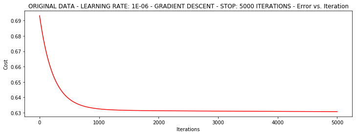
设定迭代次数
#选择的梯度下降方法是基于所有样本的
n=100
runExpe(orig_data, theta, n, STOP_ITER, thresh=5000, alpha=0.000001)
***Original data - learning rate: 1e-06 - Gradient descent - Stop: 5000 iterations
Theta: [[-0.00027127]
 [ 0.00705232]
 [ 0.00376711]] - Iter: 5000 - Last cost: 0.63 - Duration: 1.65s


array([[-0.00027127],
       [ 0.00705232],
       [ 0.00376711]])
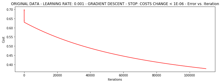
根据损失值停止
设定阈值为1E-6
runExpe(orig_data, theta, n, STOP_COST, thresh=0.000001, alpha=0.001)
***Original data - learning rate: 0.001 - Gradient descent - Stop: costs change < 1e-06
Theta: [[-5.13364014]
 [ 0.04771429]
 [ 0.04072397]] - Iter: 109901 - Last cost: 0.38 - Duration: 48.19s


array([[-5.13364014],
       [ 0.04771429],
       [ 0.04072397]])
对比不同的梯度下降法
Stochastic descent
runExpe(orig_data, theta, 1, STOP_ITER, thresh=5000, alpha=0.001)
***Original data - learning rate: 0.001 - Stochastic descent - Stop: 5000 iterations
Theta: [[-0.39554857]
 [ 0.02237485]
 [-0.0276303 ]] - Iter: 5000 - Last cost: 0.89 - Duration: 0.76s


array([[-0.39554857],
       [ 0.02237485],
       [-0.0276303 ]])
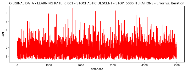
有点爆炸。。。很不稳定,再来试试把学习率调小一些
runExpe(orig_data, theta, 1, STOP_ITER, thresh=15000, alpha=0.000002)
***Original data - learning rate: 2e-06 - Stochastic descent - Stop: 15000 iterations
Theta: [[-0.00202176]
 [ 0.01001261]
 [ 0.00091419]] - Iter: 15000 - Last cost: 0.63 - Duration: 1.86s


array([[-0.00202176],
       [ 0.01001261],
       [ 0.00091419]])
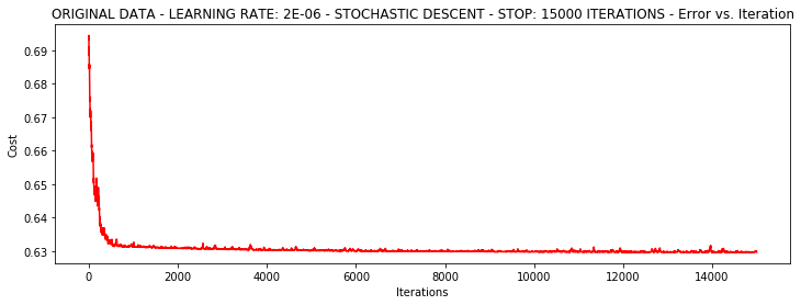
速度快,但稳定性差,需要很小的学习率
Mini-batch descent
runExpe(orig_data, theta, 16, STOP_ITER, thresh=15000, alpha=0.001)
***Original data - learning rate: 0.001 - Mini-batch (16) descent - Stop: 15000 iterations
Theta: [[-1.03466277]
 [ 0.02768388]
 [ 0.01858675]] - Iter: 15000 - Last cost: 0.72 - Duration: 2.89s


array([[-1.03466277],
       [ 0.02768388],
       [ 0.01858675]])

浮动仍然比较大,我们来尝试下对数据进行标准化 将数据按其属性(按列进行)减去其均值,然后除以其方差。最后得到的结果是,对每个属性/每列来说所有数据都聚集在0附近,方差值为1
from sklearn import preprocessing as pp

scaled_data = orig_data.copy()
scaled_data[:, 1:3] = pp.scale(orig_data[:, 1:3])

runExpe(scaled_data, theta, n, STOP_ITER, thresh=5000, alpha=0.001)
***Scaled data - learning rate: 0.001 - Gradient descent - Stop: 5000 iterations
Theta: [[0.3080807 ]
 [0.86494967]
 [0.77367651]] - Iter: 5000 - Last cost: 0.38 - Duration: 2.30s


array([[0.3080807 ],
       [0.86494967],
       [0.77367651]])
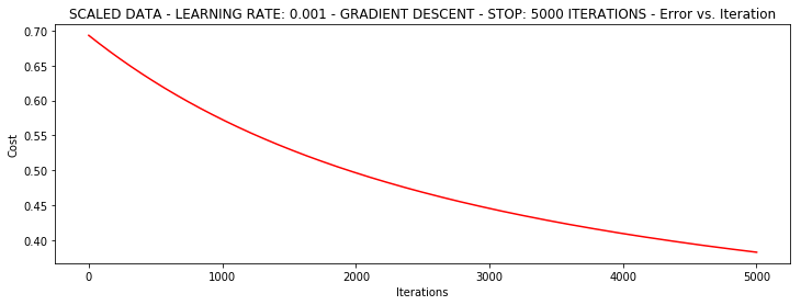
它好多了!原始数据,只能达到达到0.61,而我们得到了0.38个在这里! 所以对数据做预处理是非常重要的
runExpe(scaled_data, theta, n, STOP_GRAD, thresh=0.02, alpha=0.001)
***Scaled data - learning rate: 0.001 - Gradient descent - Stop: gradient norm < 0.02
Theta: [[1.0707921 ]
 [2.63030842]
 [2.41079787]] - Iter: 59422 - Last cost: 0.22 - Duration: 31.39s


array([[1.0707921 ],
       [2.63030842],
       [2.41079787]])

更多的迭代次数会使得损失下降的更多!
theta = runExpe(scaled_data, theta, 1, STOP_GRAD, thresh=0.002/5, alpha=0.001)
***Scaled data - learning rate: 0.001 - Stochastic descent - Stop: gradient norm < 0.0004
Theta: [[1.14837004]
 [2.7936333 ]
 [2.5646749 ]] - Iter: 72578 - Last cost: 0.22 - Duration: 13.34s
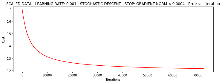
随机梯度下降更快,但是我们需要迭代的次数也需要更多,所以还是用batch的比较合适!!!
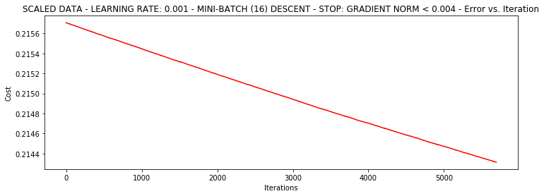
runExpe(scaled_data, theta, 16, STOP_GRAD, thresh=0.002*2, alpha=0.001)
***Scaled data - learning rate: 0.001 - Mini-batch (16) descent - Stop: gradient norm < 0.004
Theta: [[1.17941228]
 [2.8498756 ]
 [2.62631998]] - Iter: 5690 - Last cost: 0.21 - Duration: 1.33s


array([[1.17941228],
       [2.8498756 ],
       [2.62631998]])
精度
#设定阈值
def predict(X, theta):
    return [1 if x >= 0.5 else 0 for x in model(X, theta)]
scaled_X = scaled_data[:, :3]
y = scaled_data[:, 3]
predictions = predict(scaled_X, theta)
correct = [1 if ((a == 1 and b == 1) or (a == 0 and b == 0)) else 0 for (a, b) in zip(predictions, y)]
accuracy = (sum(map(int, correct)) % len(correct))
print ('accuracy = {0}%'.format(accuracy))
accuracy = 89%