OpenCV-Python系列之对极几何

点击查看代码

import numpy as np
import cv2 as cv
img1=cv.imread("data1/1.png",0) # queryimage  left image
img2=cv.imread("data1/2.png",0) # trainimage right image
sift=cv.SIFT_create()
# sift1=cv.xfeatures2d.SIFT_create()

kp1,des1=sift.detectAndCompute(img1,None)
kp2,des2=sift.detectAndCompute(img2,None)

# FLANN parameters
FLANN_INDEX_KDTREE=1
index_params=dict(algorithm=FLANN_INDEX_KDTREE,trees=5)
search_params=dict(checks=50)
flann=cv.FlannBasedMatcher(index_params,search_params)
matches=flann.knnMatch(des1,des2,k=2)
good=[]
pts1=[]
pts2=[]
# ratio test as per Lowe's paper
for i,(m,n) in enumerate(matches):
    if m.distance<0.8*n.distance:
        good.append(m)
        pts2.append(kp2[m.trainIdx].pt)
        pts1.append(kp1[m.queryIdx].pt)

现在得到了一个匹配点列表，我们就可以使用它来计算基础矩阵了。 retval,mask=cv.findFundamentalMat(points1,points2,method,ransacReprojThreshold,confidence,mask) points1: 从第一张图片开始的N个点的数组，点坐标应该是浮点数(单精度或双精度). points2: 与点1大小和格式相同的第二图像点的数组。 method: 计算基本矩阵的方法。 cv2.FM_7POINT for a 7-point algorithm.N=7 cv2.FM_8POINT for a 8-point algorithm.N>=8 cv2.FM_LMEDS for the LMedS algorithm.N>=8 ransacReprojThreshold:仅用于RANSAC方法的参数，默认3.它是一个点到极线的最大距离(以像素为单位),超过这个点就被认为是一个离群点， 不用于计算最终的基本矩阵。根据点定位、图像分辨率和图像噪声的准确性，可以将其设置为1-3左右。 confidence:仅用于RANSAC和LMedS方法的参数，默认0.99。它指定了一个理想的置信水平(概率),即估计矩阵是正确的

点击查看代码

pts1=np.int32(pts1)
pts2=np.int32(pts2)
F,mask=cv.findFundamentalMat(pts1,pts2,cv.FM_LMEDS)
print("F矩阵")
print(F)
# we select only inlier points
pts1=pts1[mask.ravel()==1]
pts2=pts2[mask.ravel()==1]

下一步我们要找到极线。我们会得到一个包含很多线的数组。 所以我们要定义一个新的函数将这些线绘制到图像中

点击查看代码

def drawlines(img1, img2, lines, pts1, pts2):
    ''' img1 - image on which we draw the epilines for the points in img2
        lines - corresponding epilines '''
    r, c = img1.shape
    img1 = cv.cvtColor(img1, cv.COLOR_GRAY2BGR)
    img2 = cv.cvtColor(img2, cv.COLOR_GRAY2BGR)
    for r, pt1, pt2 in zip(lines, pts1, pts2):
        color = tuple(np.random.randint(0, 255, 3).tolist())
        x0, y0 = map(int, [0, -r[2]/r[1]])
        x1, y1 = map(int, [c, -(r[2]+r[0]*c)/r[1]])
        img1 = cv.line(img1, (x0, y0), (x1, y1), color, 1)
        img1 = cv.circle(img1, tuple(pt1), 5, color, -1)
        img2 = cv.circle(img2, tuple(pt2), 5, color, -1)
    return img1, img2

现在我们两幅图像中计算并绘制极线. lines=cv.computeCorrespondEpiline(points,whichImage,F,lines) points:输入点。类型为CV_32FC2NX1或1XN矩阵。 whichImage:包含点的图像(1或2)的索引 F:基本矩阵，可使用findFundamentalMat或StereoRectify进行估计。 lines:对应于另一幅图像中的极线的输出向量(a,b,c)表示ax+by+c=0 Find epilines corresponding to points in right image(second image) and drawing its lines on left image

点击查看代码

lines1=cv.computeCorrespondEpilines(pts2.reshape(-1,1,2),2,F)
lines1=lines1.reshape(-1,3)
img5,img6=drawlines(img1,img2,lines1,pts1,pts2)
# Find epilines corresponding to points in left image(first image) and  drawing its lines on right image
lines2=cv.computeCorrespondEpilines(pts1.reshape(-1,1,2),1,F)
lines2=lines2.reshape((-1,3))
img3,img4=drawlines(img2,img1,lines2,pts2,pts1)
# plt.subplot(1,2,1), plt.imshow(img5)
# plt.subplot(1,2,2), plt.imshow(img3)
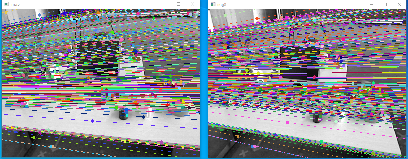
cv.imshow("img5",img5)
cv.imshow("img3",img3)
cv.waitKey(0)

我们可以在左侧图像中看到所有Epilines都在右侧图像的一点处收敛。那个汇合点就是极点。