python matplotlib

import matplotlib as mpl
mpl.get_backend()
# 'nbAgg'
import matplotlib.pyplot as plt

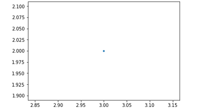
plt.plot(3,2,'.')

作图 :

 

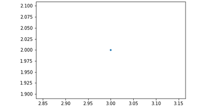
from matplotlib.backends.backend_agg import FigureCanvasAgg
from matplotlib.figure import Figure

fig = Figure()
canvas = FigureCanvasAgg(fig)

ax = fig.add_subplot(111)
ax.plot(3, 2, '.')
canvas.print_png('test.png')
##notebook 中用html显示图片

%%html
<img src = 'test.png'/>

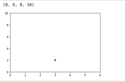
2. 用plt.gca()用法

plt.figure()
plt.plot(3, 2, 'o')
ax = plt.gca()
ax.axis([0,6,0,10])

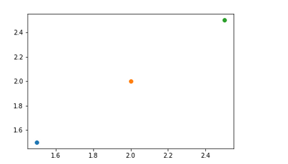
plt.figure()
plt.plot(1.5,1.5,'o')
plt.plot(2,2,'o')
plt.plot(2.5,2.5,'o')

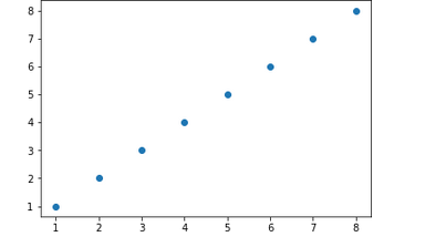
3. Scatterplot()

import numpy as np
x = np.array([1,2,3,4,5,6,7,8])
y = x
plt.figure()
plt.scatter(x,y)

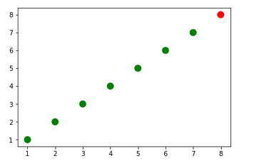
import numpy as np
x = np.array([1,2,3,4,5,6,7,8])
y = x
colors = ['green']*(len(x)-1)
colors.append('red')

plt.figure()
plt.scatter(x,y,s=100, c=colors) #s为scatter 点的size

zip()

zip_generator = zip([1,2,3,4,5],[6,7,8,9,10])
list(zip_generator)
"""
output: 
[(1, 6), (2, 7), (3, 8), (4, 9), (5, 10)]

"""

zip_generator =  zip([1,2,3,4,5],[6,7,8,9,10])
#unpack this result into two variables directly ,x ans y
x,y = zip(*zip_generator) 
print(x)
print(y)
#output:
# (1, 2, 3, 4, 5)
# (6, 7, 8, 9, 10)
#

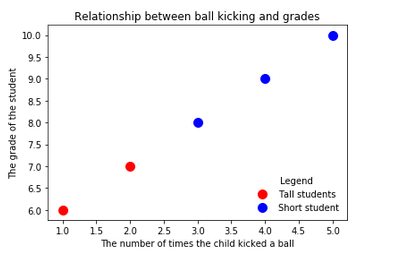
散点图画法

plt.figure()
plt.scatter(x[:2], y[:2], s=100, c='red',  label='Tall students')
plt.scatter(x[2:], y[2:], s=100, c='blue', label ='Short student')

plt.xlabel('The number of times the child kicked a ball')
plt.ylabel('The grade of the student')
plt.title('Relationship between ball kicking and grades')

plt.legend()

plt.legend(loc=4, frameon=False, title='Legend') #右下角

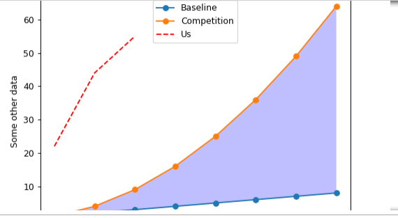
 4. Linear plot

import numpy as np
linear_data = np.array([1,2,3,4,5,6,7,8])
quadratic_data = linear_data**2

plt.figure()
plt.plot(linear_data, '-o', quadratic_data, '-o')

plt.plot([22,44,55], '--r')

plt.xlabel('Some data')
plt.ylabel('Some other data')
plt.title('A title')
plt.legend(['Baseline', 'Competition', 'Us'])

#fill
plt.gca().fill_between(range(len(linear_data)),
                      linear_data, quadratic_data,
                      facecolor='blue',
                      alpha = 0.25)

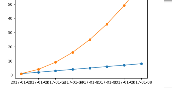
plt.figure()

observation_dates = np.arange('2017-01-01', '2017-01-09', dtype='datetime64[D]')

plt.plot(observation_dates, linear_data, '-o', observation_dates, quadratic_data,'-o')

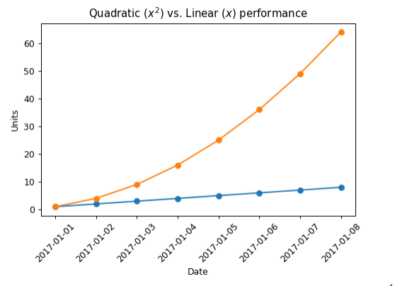
plt.figure()
observation_dates = np.arange('2017-01-01','2017-01-09', dtype='datetime64[D]')
observation_dates = list(map(pd.to_datetime, observation_dates))
plt.plot(observation_dates, linear_data, '-o', 
         observation_dates, quadratic_data, '-o')

x = plt.gca().xaxis

for item in x.get_ticklabels():
    item.set_rotation(45) #旋转一定的角度
    
plt.subplots_adjust(bottom=0.25) #调整与底部的距离

ax = plt.gca()
ax.set_xlabel('Date')
ax.set_ylabel('Units')
ax.set_title('Quadratic vs. Linear performance')

ax.set_title('Quadratic ($x^2$) vs. Linear ($x$) performance' ) #Latex

5 .  Bar chart

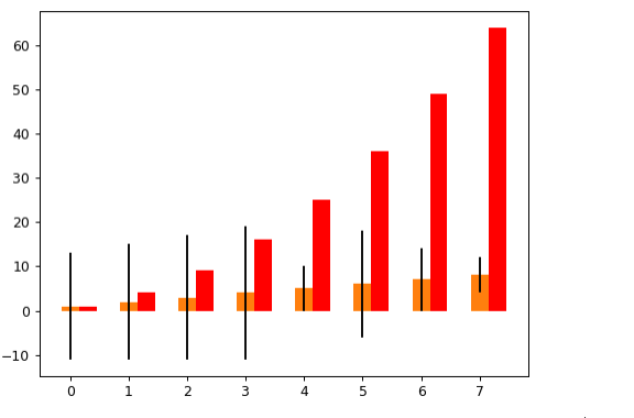
plt.figure()
xvals = range(len(linear_data))
plt.bar(xvals, linear_data, width=0.3)

new_xvals = []
for item in xvals:
    new_xvals.append(item+0.3)

plt.bar(new_xvals, quadratic_data, width=0.3, color='red')

from random import randint
linear_err = [randint(0,15) for x in range(len(linear_data))]
plt.bar(xvals, linear_data, width=0.3, yerr = linear_err)

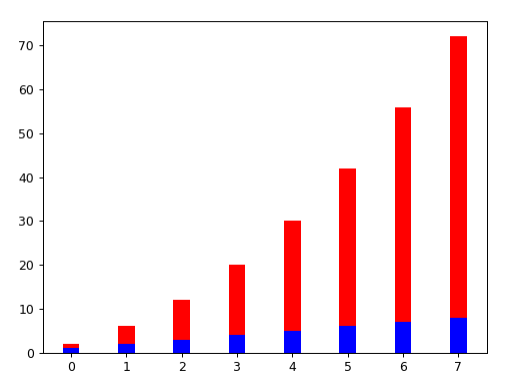
plt.figure()
xvals = range(len(linear_data))
plt.bar(xvals, linear_data, width=0.3, color='b')
plt.bar(xvals, quadratic_data, width=0.3, bottom = linear_data,color='r')

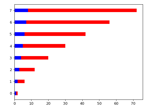
plt.figure()
xvals = range(len(linear_data))
plt.barh(xvals, linear_data, height=0.3, color='b')
plt.barh(xvals, quadratic_data, height=0.3, left=linear_data, color='r')
#垂直变水平