Principle of AI 学习笔记

Introduction

Terminology

NP-completeness: In computational complexity theory
- P: Polynomial time
- NP: Non-deterministic Polynomial time
- NP-complete: the conjunction of NP and NP-hard

Definition

the intelligence exhibited by machines or software
the name of the academic field of research
how to create computers and compter software that are capable of intelligent behaviour

Certification

Turing test: designed to provide a satisfactory operational definition of intelligence
- a computer passes the test if a human iterrogator, after posing some written questions, can not tell whether the written responses come from a person of from a computer
- Turing prediction: by the year 2000, machines would be capable of fooling 30% of human judges after five minutes of questioning
visual Turing test: an operator assisted device that produces a stochastic sequence of binary questions from a given test image
- motivated by the ability of human to understand images
Chinese Room: a thought experiment attempts to show that computer can never be properly described as having a "mind" or "understanding", regardless of how intelligently it maybe have
- He understands nothing of Chinese, and yet, by following the program for manipulating symbols and numerals just as a computer does, he produces appropriate strings of Chinese characters that fool those outside into thinking there is s Chinese speaker in the room

Foundation

Philosophy
Mathematics
- logic (What are the formal rules to draw valid conclusions)
- computation (What can be computed)
- probability (How do we reason with uncertain information)
Economics
Neuroscience (How do brains process information)
Psychology (cognitive psychology) (How do hummans think and act):
- attention: a state of focused awareness on a subset of available percoptual information
- language use: study language acquisition, individual components of language formation, how language use is involved in mood, or numerous other related areas
- memory
  - procedural memory
  - semantic memory
  - episodic memory
- perception: Physical senses(sight,smell,hearing,taste,touch and proprioception), as well as their cognitive processes
- problem solving
- creativity
- thinking
- metacognition: cognition about cognition/thinking about thinking/knowing about knowing
  - knowledge about cognition
  - regulation of cognition
- vs. cognitive science:
  - cognitive psychology: be often involved in running psychological experiments involving human participants, with the goal of gathering information related to how the human mind takes in, processes and acts upon inputs received from the outside world
  - cognitive science: be concerned with gathering data through research, which has links to phil;osophy, linguistics, anthropology, neuroscience and particularly with AI
Computer engineering
Control theory and cybernetics (how can artifacts operate under their own control)
- control theory: an interdisciplinary branch of engineering and mathematics (Deal with the behavior of dynamical systems with inputs, and how their behaviour is modified by feedback)
- cybernetics:
  - a transdisciplinary approach of exploring regulatory systems, their structures, constraints and possibilities
  - the scientific study of control and commnication in the animal and the machine
  - control of any system using technology
Linguistics

History of AI

1950-1956: the birth of AI
- 1950: the birth of Turing Test
- 1956: AI research was founded
1956-1974: the golden years
- 1958: the first AI program, Logic Theorist (LT)
- 1958: Lisp programming language
- 1960s: semantic nets
- 1963: one of the first ML programs in "A Pattern Recognition Program That Generates, Evaluates, and Adjusts Its Own Operators"
- 1965: the first expert system, Dendral (a software to deduce the molecular structure of organic components)
- 1974: MYCIN program (a very practical ruole-based approach to medical diagnoses)
1974-1980: the first AI winter
- 1966: the failure of machine translation
- 1970: the abandonment of connectionism
- 1973-1974: the large decrease in AI research in U.K. and U.S.
1980-1987: the boom of AI
- 1980：the first national conference of AAAI held
- 1982: FGCS started for knowledge processing
- mid-1980s: decision tree and ANN
1987-1993: the second AI winter
- 1987: the collapse of the Lisp machine market
- 1988: the decrease in AI spending in U.S.
- 1993: expert systems slowly reaching the bottom
- 1990s: the quiet disappearance of the FGCS's original goals
1993-present: the breakthrough
- 1997: the first computer chess-playing system, Deep Blue, beat Garry Kasparov
- 2005: Stanley, an autonomous robotic vehicle, won the DARPA Grand Challenge
- 2006: "deep learning
- 2011: Google Brain
- 2012: Apple's Siri
- 2012: a real-time English-to-Chinese universal translator that keeps your voice and accent
- Apr. 2014: Microsoft's Cortana
- Jun. 2014: Microsoft China's XiaoIce
- Jun. 2014: chatbot Eugene Goostman passed the Turing Test
- Aug. 2014: IBM's TrueNorth chip
- Feb. 2015: Deep Q-Network
- Dec. 2015: AlphaGo beat the European Go champion
- Mar. 2016: AlphaGo beat Lee Sedol
- some other good AIs:
  - Watson: for quiz show Jeopardy
some opposite voice:
- Jan. 2016: the Information Technology and Innovation Foundation (ITIF) in Washington DC announced its annual Luddite Award. ITIF gave the Luddite Award to “a loose coalition of scientists and luminaries who stirred fear and hysteria in 2015 by raising alarms that artificial intelligence (AI) could spell doom for humanity”

The state of Art

the categories of AI:
- divide standard:
  - humanly/rationally:
    - humanly: to measure success in terms of fidelity to human performance
    - rationally: to measure against an ideal performance measure
  - acting/humanly
  - Weak/Strong/Super AI:
    - Weak AI (Artificial Narrow Intelligence/ANI): non-sentient AI that is focused on one narrow task (just a specific problem)
    - Strong AI (Artificial General Intelligence/AGI): a machine with the ability to apply intelligence to any problem (a primary goal of AI research)
    - Super AI (Artificial Super Intelligence/ASI):
      - a hypothetical agent that possesses intelligence far surpassing that of the brightest and most gifted human minds
      - a property of problem-solving systems (super intelligent language translators/engineering assistants)
- definitions for four categories:
  - acting humanly:
    - to perform functions that require intelligence performed by people
    - to make computers do things at which, at the moment, people are better
  - acting rationally:
    - computational intelligence is the study to design intelligent agent
    - AI is concerned with intelligent behaviour in artifacts
  - thinking humanly:
    - the automation of activities that we associate with human thinking ...
    - the new effort to make computers think ... machine with minds ...
  - thinking rationally:
    - the study of mental faculties through the use of computational models
    - to make computer possible to perceive, reason and act
the application of AI:
- Typical problems:
  - Computer Vision(CV)
  - Image processing
  - XR(AR,VR,MR)
  - pattern recognition
  - intelligent diagnosis
  - Game theory and Strategic planning
  - Game AI and Gamebot
  - Machine Translation
  - Natural Language Processing(NLP)
    - chatbot
  - nonlinear control (Robotics)
- other fields:
  - Artificial life
  - Automated reasoning
  - Biological computing
  - concept mining
  - data mining
  - knowledge representation
  - Semantic Web
  - Emai spam filtering
  - Litigation
  - Robotics
    - Behaviour-based robotics
    - cognitive
    - cybernetics
    - development robotics
  - hybrid intelligent system
  - intelligent agent
  - intelligent control
Typical papers on AI:
- "A Global Geometric Framework for Nonlinear Dimensionality Reduction". SCIENCE, Vol. 290, Dec. 2000
- "Nonlinear Dimensionality Reduction by Locally Linear Embedding". SCIENCE, Vol. 290, Dec. 2000
- "Reducing the Dimensionality of Data with Neural Networks". SCIENCE, Vol. 313, Jul. 2006
- "Clustering by fast search and find of density peaks". SCIENCE, Vol. 344, Jun. 2014
- "Human-level concept learning through probabilistic program induction". SCIENCE, Vol. 350, Dec. 2015
- "Human-level control through deep reinforcement learning". NATURE, Vol. 518, Feb. 2015
- "Deep learning". NATURE, Vol. 521, May. 2015
- "Mastering the game of Go with deep neural networks and tree search". NATURE, Vol. 529, Jan. 2016
research area of AI:
- searching: problem space
- reasoning: knowledge
- planning: rules
- learning: data
- applying:
  - communicating: NLP, Machine Trans.
  - perceiving: vision, speech, sensing
  - acting: robot

Intelligent Agent

Approaches for AI

Cybernetics and Brain Simulation (Soar)
symbolic & sub-symbolic
- symbolic AI: based on high-level "symbolic"(human-readable) representations of problems, logic and search
  - base: assumption taht many aspects of intelligence can be achieved by the manipulation of symbols
  - most successful form: expert systems
- sub-symbolic AI:
  - basis: NN, statistics, numerical optimization, etc.
logic-based vs. anti-logic
- logic-based: machines did not need to simulate human thought, but should instead try to find the essence of abstract reasoning and problem solving, regardless of whether people used the same algorithms
  - Prolog(a programming language), logic programming
- anti-logic: argue that there was no simple and general pinciple (like logic) to capture all the aspects of AI
  - commomsense knowledge bases
  - knowledge-based (knowledge revolution) (result in the development and deployment of expert systems)
symbolism vs. connctionism
- symbolist AI: represents information through symbols and their relationships (specific algorithms are used to process these symbols to solve problems or deduce new knowledge)
- connectionist AI: represents information in a distributed form within a network (imitates biological processes underlying learning, task performance and problem solving)
statistical approach: sophisticated mathematical tools to solve specific sub-problems
- critics: these techniques are too focused on particular problems and have failed to address the long term goal of general intelligence
intelligent agent paradigm:
- factors need to satisfy:
  - operate autonomously
  - perceive their environment
  - persist over a prolonged time period
  - adapt to change
  - create and pursue goals
  - the best outcome/the best expected outcome
- broadly, an agent is anything that can be viewed as:
  - perceiving its environment through sensors and acting upon that environment through actuators
  - may also learn or use knowledge to achive their goals
- example: human agent/robotic agent/software agent

Rational Agent

Why:
- more general than the "thinking/acting humanly" approaches, because correct inference is just one of several ppossible mechanisms for achieving rationality
- more amenable to scientific development than the "thinking/acting humanly" approaches
abstrct intelligent agents: a concept developed to describe computer program agents and distinguish them from their real world ones as computer systems, biological systems or organizations
- other descriptions: autonomous intelligent agent, rational agent
- a variety of definitions:
  - accommodate new problem solving rules incrementally
  - adapt online and inreal time
  - able to analyze itself in terms of behavior, error and success
  - learn and improve through interaction with the environ ment
  - learn quickly from large amounts of data
  - having parameters to present short and long term memory, forgetting, etc.
- example: vacuum-cleaner world
what's a rational agent: one that does the right thing —— every entry in the table for thw agent function is filled out correctly
- what's the right thing:
  - An agent in an environment generates a sequence of actions according to the percepts. Those actions causes the environment to go through a sequence of states. If the sequence is desirable, then the agent has performed well
- rational: exploration, learning, autonomyy
- rational action(=right thing): maximizes the expected value of performance measure given the percept sequence
  - rational $=$ best $=$ optimal $\neq$ omniscience $\neq$ clairvoyant $\neq$ successful
concept of rationality: rationality depends on four things:
- the performance measure that defines the criterion of success
- the agent;s prior knowledge of the environment
- the actions that the agent can perform
- the agent's percept sequence to date

Task Environments

PEAS description: a task environment specification
- Performance
- Environment
- Actuators
- Sensors
Environment types:
- fully observable vs. partially observable
  - fully observable: an agent's sensors give it access to the complete state of the environment at each point in time
  - partially observable: an agent's sensors can only give it access to part of the state of the environment at each point in time
- single agent vs. multi-agent
  - single agent: an agent operating by itself in an environment
  - multi-agent: many agents operating in the same environment
- deterministic vs. stochastic
  - deterministic: the next state of the environment is completely determined by the current state and the action executed by the agent
  - stochastic: the next state of the environment is not or partly determined by the current state and the action executed by the agent
- episodic vs. sequential
  - episodic: the agent;s experience is divided into atomic episodes and the thoice of action in each episode depends only on the episode itself
  - sequential: the agent;s experience is divided into atomic episodes and the thoice of action in each episode depends on the episode itself and the episodes ahead
- dynamic vs. static:
  - dynamic: the environment can change while an agent is deliberating
  - static: the environment can't change while an agent is deliberating
  - semi-dynamic: the environment itself does not change with the passage of time but the agent's performance score does
- discrete vs. continuous:
  - discrete: the state of the environment, the way time is handled and the percpets and actions of the agent is discrete
  - continuous: the state of the environment, the way time is handled and the percpets and actions of the agent is continuous
- known vs. unknown:
  - known: In a known environment, the outcomes for all actions are given
  - unknown: In a known environment, the outcomes for all actions are not given
    (If the environment is unknown, the agent will have to learn how it works in order to make good decisions)

Intelligent Agent Struture

description: an agent function $f:{\cal P^* \rightarrow A}\ \ {\sf where}\ \ {\cal P^*}=\sum\limits_{t=1}^T|{\cal P}|^t$
- agent function: an abstrct concept that incorporates various principles of decision making
  - calculation of utility of individual options
  - deduction over logic rules
  - fuzzy logic
  - lookup table
  - etc.
- agent program: the programming implementation of an agent function
the structure of agents:
- platform
  - computing device
  - sensors
  - actuators
- agent program $\supset$ agent function
three ways to present states for an agent:
- atomic: each state is a black box with no internal structure
- factored: each state consists of a fixed set of attributes and values
- structured: each state includes objects, each has attributes and relationships to other objects

Category of Intelligent Agents (based on the degree of perceived intelligenve and capability)

simple reflex agents
- feature:
  - act only on the basis of the current percept,ignoring the rest of the percept history
  - agent function is based on condition-action rule (if-then)
- structure:
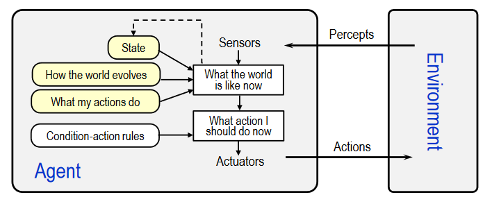
- something about simple reflex agents:
  - Succeeds only when the environment is fully observable
  - Some reflex agents can also contain information on their current state which allows them to disregard condition whose actuators are already triggered
  - Infinite loops are often unavoidable for agents operating in partially abservable environments
    - Note: If the agent can randomize its actions, it may be possible to escape from infinite loops
- program implementation:
  - state: the agent's current conception of the world state
  - rules: a set of condition-action rules
  - action: the most recent action (initially none)
```
def simple_reflex_agent(percept):
  state=interpret_input(percept)
  rule=rule_match(state,rules)
  action=rule.action
  return action
```
model-based reflex agents
- feature:
  - can handle partially observable environment
  - Its current state is stored inside the agent maintaining some kind of structure which describes the part of the world which cannot be seen
- structure:
- something about model-based reflex agents:
  - This knowledge about "how the world works" is called a model of the world
  - A model-based reflex agent should maintain some sort of internal model
  - The internal model depends on the percept history and thereby reflects at least some of the unobserved aspects of the current state. It then chooses an action in the same way as the reflex agent.
- program implementation:
  - state: the agent's current conception of the world state
  - model: a description of how the next state depends on current state and action
  - rules: a set of condition-action rules
  - action: the most recent action (initially none)
```
def model_based_reflex_agent(percept):
  state=update_state(state,action,percept,model)
  rule=rule_match(state,rules)
  action=rule.action
  return action
```
goal-based agents
- feature: further expand on the capabilities of the model-based agents by using "goal" information
- structure:
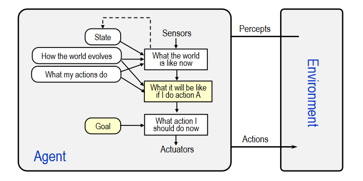
- something about goal-based agents:
  - goal information: describes situations that are desirable
    (This allows the agent a way to choose among multiple possibilities, selecting the one which reaches a goal state)
  - Search and planning are the subfields of AI devoted to finding action sequences that achieve the agent's goals
  - In some instances the goal-based agent appears to be less efficient, but it's more flexible because the knowledge that supports its decisions is represented explicitly and can be modified
utility-based agents
- feature: A particular state can be obtained by a utility function which maps a state to a measure of the utility of the state
- structure:
- something about utility-based agents
  - utility: used to describe how happy the agent is
    (A more general performance measure should allow a comparison of different world states according to exactly how "happy" they would make the agent)
  - A rational utility-based agent chooses the action that maximizes the expected utility of the action outcomes
  - A utility-based agent has to model and keep track of its environment, tasks that have involved a great deal of research on perception, representation, reasoning and learning
learning agents
- feature: Learning allows the agents to initially operate in unknown environments and to become more competent than its initial knowledge
- structure:
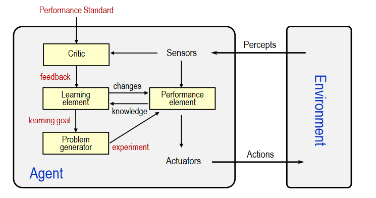
- something about learning agents:
  - learning element:
    - It uses feedback from the "Critic" on how the agent is doing, and determines how the performance element should be modified to do better in the future
  - performance element:
    - It is what we have previously considered to be the eentire agent: it takes in percepts and decides on actions
  - problem generator:
    - It is responsible for suggesting actions that will lead to new experiences
other agents:
- decision agents: agents geared to decision making
- input agents: agents process and make sense of sensor inputs
- processing agents: agents solve a problem like speech recognition
- spatial agents: agetns relate to the physical real-world
- temporal agents: agents may use time based stored information to offer instructions(or data acts) to a computer program(or human being), and takes program inputs percepts to adjust its next behaviors
- world agents: agents incorporate a combination of all the other agents to allow autonomous behaviors
- believable agents: agents exhibiting a personality via the use of an artificial character (the agent is embedded) for the interaction
real cases:
- shopping agent
- customer help desk
- personal agent
- data-mining agent
a perspective for agents:
- multiple $+$ learning $=$ multiple learning agents
- multiple $+$ autonomous $=$ multiple agents
- autonomous $+$ learning $=$ interface agents
- multiple $+$ autonomous $+$ learing $=$ intelligence agents
A Taxonomy of Agents:
- intelligent agents
  - biological agents
  - robotic agents
  - computational agents
    - single agents
      - simple agents
      - model-based agents
      - goal-based agents
      - utility-based agents
      - learning agents
      - other
    - multiple agents

Searching

defs

Problem solving agent:
- defs:
  - solution: a seq of actions to reach the goal
  - process: look for the seq of actions, which is called search
  - problem formulation: given a goal, decide what actions and states to consider
- why search: some NP-complete or NP-hard problems can be solved only by search
- problem-solving agent: a kind of goal-based agent to solve problems through search
- algorithm:
  - seq: a action sequnce, initially empty
  - state: some description of the current world state
  - goal: a goal, initially NULL
  - problem: a problem formulation
  - action: the most recent action, initially none
```
def simple_problem_solving_agent(percept):
  state=update_state(state,percept)
  if seq.empty():
    goal=formulate_goal(state)
    problem=formulate_problem(state,goal)
    seq=search(problem)
    if seq==failure return NULL
  action=first(seq)
  seq=rest(seq)
  return action
```
related terms:
- state space: defined by initial state, actions and transition model
  - initial state: the agent starts in
  - actions: a description of the possible actions available to the agent
  - transition model: a description of what each action does
  - goal test: to determine whether a given state is a goal state
  - path cost: to assign a numeric cost to each path
- graph: state space forms a graph, in which nodes are states, and links are actions
- path: a seq of states connected by a seq of actions
search type:
- classical search: the search above problems whose solution is a sequence of actions that are observable, deterministic with known environments (search space systematically)
  - uninformed search
  - informed search
- local search
- swarm intelligence

searching for solutions

tree-search algorithm:

def tree_search(problem):
  frontier=init(problem.initial_state)
  while True:
    if frontier.empty() return failure
    now=choose_a_leaf(frontier)
    frontier.remove(now)
    if now.contain(goal_state) return now.solution
    frontier.add(now.resulting_nodes)

graph-search algorithm:

def graph_search(problem):
  frontier=init(problem.initial_state)
  explored.clear()
  while True:
    if frontier.empty() return failure
    now=choose_a_leaf(frontier)
    frontier.remove(now)
    if now.contain(goal_state) return now.solution
    explored.add(now)
    for node in now.resulting_nodes:
      if not frontier.has(node) and not explored.has(now):
          frontier.add(now)

def: the search strategies that have no additional information about states beyond that provided in the problem definition
- All they can do is to generate successors and distinguish a goal state from a non-goal state
evaluation:
- completeness (Does it always find a solution if one exists)
- time complexity (How long does it take to find a solution)
- space complexity (How much memory is needed)
- optimality (does it always find the optimal solution)
some factors:
- b: the maximum branching factor of the search tree
- d: depth of the shallowest solution
- m: maximum depth of the search tree

divisions: (by the order in which nodes are expanded)

breadth-first search(BFS): expand the shalloewest unexpanded node first

time complexity: $O(b^d)$ (major factor)
space complexity: $O(b^d)$

def bfs(problem):
  node=Node(state=problem.initial_state)
  path_test=0
  frontier=Queue(elements=node)
  explored=Set()
  while True:
    if frontier.empty() return failure
    node=frontier.pop()
    explored.add(node.state)
    for action in problem.actions(node.state):
      child=child_node(problem,node,action)
      if not explored.has(child.state) and not frontier.has(child.state):
          if problem.goal_test(child.state) return solution(child)
          frontier.push(child)

depth-first search(DFS): expand deppest unexpanded node first
- time complexity: $O(b^m)$
- space complexity: $O(bm)$

uniform-cost search: expand lowest-cost unexpanded node

time complexity: $b^{1+\lfloor\frac{C^*}\epsilon\rfloor}$
space complexity: $b^{1+\lfloor\frac{C^*}\epsilon\rfloor}$

def uniform_first_search(problem):
  node=Node(state=problem.initial_state)
  path_test=0
  frontier=PriorityQueue(elements=node)
  explored=Set()
  while True:
    if frontier.empty() return failure
    node=frontier.pop()
    if problem.goal_test(node.state) return solution(node)
    explored.add(node.state)
    for action in problem.actions(node.state):
      child=child_node(problem,node,action)
      if not frontier.has(child.state) and not explored.has(child.state):
        frontier.push(child)
      else if frontier.has(child.state) and frontier[child.state]<child.path_cost:
          frontier[child.state]=child.path_cost

optimized akgorithms:
- depth-limite search:
  - optimization: nodes at depth l are treated as if they hace no successors
  - disadvantage:
    - introduce an additional source of incompleteness if we choose $l<d$
    - non-optimal if we choose $l>d$
  - time complexity: $O(b^l)$
  - space complexity: $O(bl)$
```
def depth_limited_search(problem,limit):
  return recursive_DLS(Node(problem.initial_state),problem,limit)
def recursive_DLS(node,problem,limit):
  if problem.goal_test(node.state) return solution(node)
  if limit==0 return cutoff
  cutoff_occured=False
  for action in problem.actions(node.state):
    child=child_node(problem,node,action)
    result=recursive_DLS(child,problem,limit-1)
    if result==cutoff cutoff_occured=True
    else if result!=failure return result
  if cutoff_occured return cutoff
  else return failure
```
- iterative deepening search: combines the benefits of depth-first and breadth-first search, running repeatedly with gradually increasing depth limits until the goal is found
  - time complexity: $O(b^d)$
  - space complexity: $O(bd)$
```
def iterative_deepening_search(problem):
    for depth in range(infty):
      result=depth_limited_search(problem,depth)
      if result!=cutoff return result
```
- bidirectional search: runs two simultaneous searches (one forward from the initial state, and another backward from the goal) (stops when the two meet in the middle) (can be guided by a heuristic estimate of the remaining distance)
  - time complexity: $O(b^{\frac d2})$
  - space complexity: $O(b^{\frac d2})$

Informed Search(Heuristic Search)

def: use problem-specific knowledge beyond the definition of the problem itself $\Rightarrow$ can find solutions more effciently than can an uninformed strategy
general approaches:
- evaluation function $f(n)$ : used to select a node for expansion
- heuristic function $h(n)$ : as a component of $f$
divisions:
- Best-first Search: a node was selected for expansion based on an evaluation function $f(n)$
  - implementation: the same as uniform-cost search ( $f(n)$ instead of $g(n)$ )
  - Greedy Search:
    - evaluation function: $f(n)=h(n)$
      - $h(n)$ : estimated cost from $n$ to the closest goal
    - why greedy: at each step it tries to get as close to the goal as it can
    - worst-case time: $O(b^m)$
    - space complexity: $O(b^m)$
  - $A^*$ search: avoid expanding expensive paths, minimizing the goal estimated solution cost
    - evaluation function: $f(n)=g(n)+h(n)$
      - $g(n)$ : cost to reach the node
      - $h(n)$ : estimated cost to get from the node to the goal
    - theorem: $A^*$ search is optimal
- iterative deepening $A^*$ search: a varient of iterative deepening depth-first search that borrows the idea to use a heuristic function to evaluate the remaining cost to get to the goal from the $A^*$ search algorithm
  - features:
    - lower memory usage than $A^*$ (a depth-first search algorithm)
    - doesn't go to the same depth everywhere in the search tree

Local Search

feature:
- the path followed by the search are not retained
- most basic local search algorithm without maintaining a search tree
advantages:
- use very little memory
- can find reasonable solutions in large or infinite(continuous) state spaces
application:
- integrated-circuit design
- factory-floor layout
- job-shop scheduling
- automatic programming
- telecommunications
- network optimization
- vehicle routing
- portfolio management
optimization:
- local search algorithms are useful for solving pure optimization problems
- aim in optimization: to find the best state according to an objective function
- but many optimization problems do not fit using the search algorithms introduced previously
evaluation:
- optimal: an optimal local search algorithm always finds a global minimum or maximum
- complete: a complete local search algorithm always finds a goal if one exists
typical algorithms:
- hill-climbing(greedy local search): a mathematical optimization technique which belongs to the family of local search
  - procedure: an iterative algorithm
    - starts with an arbitraty solution to a problem
    - then incrementally change a single element of the solution
    - if it's a better solution, the change is made to the new solution
    - repeating until no further improvements can be found
  - implementation: (steepest-ascent version)
    - current: a node
    - neighbour: a node
```
def hill_climbing(problem):
    current=Node(problem.initial_state)
    while True:
      neighbor=a_successor_of(current)
      if neighbor.value<=curent.value return current.state
      current=neighbour
```
  - weakness: often get stuck for the tree reasons:
    - local maxima
    - plateaux
    - ridges
  - variants of hill-climbing:
    - stochastic hill-climbing: chooses at random among uphill moves
      - the probability of selection can vary with the steepness of uphill move
      - this usually converges more slowly than steepest ascent
    - first-choice hill-climbing: implements stochastic hill climbing by generating successors randomly until one is generated that is better than the current state
      - is a good strategy when a state has many of successors
    - random-restart hill-climbing: conducts a series of hill-climbing searches from randomly generated initial states, until a goal is found
      - It is trivially complete with probability approaching 1, because it will eventually generate a goal state as the initial state
      - If each hill-climbing search has a probability $p$ of success, then the expected number of restarts required is $\frac 1p$
- local beam search: keep track of $k$ states rather than just $1$
  - procedure:
    - begins with $k$ randomly generated states
    - at each step, all the successors of all $k$ states are generated
    - If anyone is a goal, the algorithm halts, else it selects the $k$ best successors from the complete list, and repeats
  - variant of local beam search: stochastic beam search:
    - problem: local beam search may quickly become concentrated in a small region of state space, making the search little more than an expensive version of hill climbing
    - optimization: instead of choosing best $k$ successors, it chooses $k$ successors randomly, with the probability of choosing a successor being an increasing function of its value
- Tabu search: a meta-heuristic algorithm, used for solving combinatorial optimization problems
  - principle: It uses a local or neighbourhood search procedure, to iteratively move from one poitential solution $x$ to an improved neighborhood solution $x'$ , until some stopping condition has been satisfied
  - tabu list: the memory structure to determine the solution is called tabu list
  - strategies:
    - forbidding strategy: control what enters the tabu list
    - freeing strategy: control what exits the tabu list and when
    - short-term strategy: manage interplay between the forbidding strategy and freeing strategy to select trial solutions
  - implementation:
```
def tabu_search(s_0)
  sBest=s=s_0
  while not stopping_condition():
    candidateList=List()
    bestCandidate=NULL
    for sCandidate in sNeighborhood:
      if not tabuList.contains(sCandidate) and fitness(sCandidate)>fitness(bestCandidate):
        bestCandidate=sCandidate
    s=bestCandidate
    if iftness(bestCandidate)>fitness(sBest):
      sBest=bestCandidate
    tabuList.push(bestCandidate)
    if tabuList.size>maxTabuSIze:
      tabuList.remove_first()
  return sBest
```
  - typical problems:
    - travelling salesperson problem
    - travelling tournament problem
    - job-shop scheduling problem
    - network loading problem
    - the graph coloring problem
    - hardware/software partitioning
    - minimum spanning tree problem
  - other application fields:
    - resource planning
    - telecommunication
    - VLSI design
    - financial analysis
    - scheduling
    - space planning
    - energy distribution
    - molecular engineering
    - logistics
    - flexible manufacturing
    - waste management
    - mineral exploration
    - biomedical exploration
    - environmental conservation
optimizations:
- simulated annealing: a probabilistic technique fro approximating the global optimum of a given function (a meta-heuristic to approximate global optimization in a large search space)
  - annealing: used to temper or harden metals and glass
  - optimization and thermodunamics:
    - objective function $\Leftrightarrow$ energy level
    - admissilble solution $\Leftrightarrow$ ssytem state
    - neighbor solution $\Leftrightarrow$ change of state
    - control parameter $\Leftrightarrow$ temperature
    - better solution $\Leftrightarrow$ solidification state
  - implementation:
    - initial solution: generated using an heuristic, chosen at random
    - neighborhood: generated randomly, mutating the current solution
    - acceptance: neighbor has lower cost value, higher cost value is accepted with the probability $p$
    - stopping criteria: solution with a lower vvalue than threshold. maximum total number of iterations.
    - problem: a problem
    - schedule: a mapping from time to "temperature"
```
def simulated_annealing(problem,schedule):
  current=Node(problem.initial_state)
  for t in range(infty):
    T=schedule(t)
    if T==0 then return current
    next=a_random_successor(current)
    DeltaE=next.value-current.value
    if DeltaE>0 then current=next
    elif p<exp(DeltaE/T) then current=next
```
- genetic algorithms: a search heuristic that mimics the process of natural selection
  - The algorithm is a variant of stochastic beam search, in which successor states are generated by combining two parent states rather than by modifying a single state (is dealing with sexual reproduction rather than asexual reproduction)
  - belonging class: evolutionary algorithms
  - feature: generate solutions to optimmization problems using techniques inspired by natural evolution, such as inheritance, mutation, selection and crossover
  - procedure:
    - begin with a set of $k$ randomly generateed states, called the population
    - each state(individual) is represented as a string over a finite alphabet, most commonly, a string of 0s and 1s
  - implementation:
    - population: a set of individuals
    - fitness-fn: a function that measures the fitness of an individual
```
def genetic_algorithm(population,fitness_fn):
  do:
    new_population=Set()
    for i in range(size(population)):
      x=random_selection(population,fitness_fn)
      y=random_selection(population,fitness_fn)
      child=reproduce(x,y)
      if randp()<small_random_probability:
        child=mutate(child)
      new_population.add(child)
    population=new_population
  while fit_enough(population) or time>time_limit
  return population.best_individual(fitness_fn)
```
  - application:
    - bioinformatics
    - computational science
    - engineering
    - economics
    - chemistry
    - manufacturing
    - mathematics
    - physics
    - phylogenetics
    - pharmacometrics

swarm intelligence

def: study of computational systems inspired by the "collective intelligence"
- collective intelligence:
  - emerges through the cooperation of large numbers of homogeneous agents in the environment
  - decentralized, self-organizing and distribute through out an environment
  - application: effective foraging for food, prey evading,. colony relocation
algorithms:
- altruism algorithm
- ant colony optimization
- bee colony algorithm
- artificial immune system
- bat algorithm
- multi-swarm optimization
- gravitational search algortihm
- glowworm swarm optimization
- particle swarm optimization
- river colony optimization
- river formation dynamics
- self-prepelled particles
- stochatics diffusion search
typical algorithm:
- ant colony optimization: inspired by the bahavior of ants (stigmergy, foraging) (used to find optimal paths in a graph)
  - concepts:
    - ants navigate from nest to food source blindly
    - shortest path is discovered via pheromone trails
    - each ant moves at random
    - pheromone is deposited on path
    - ants detect lead ant's path, inclined to follow
    - more pheromone on path increases probability of path being followed
  - algorithm:
    - virtual "trail" accumulated on path segments
    - starting a node selected at random
    - the path selected at random: based on amout of "trail" present on possible paths from starting node, higher probability for paths with more "trail"
    - ant reaches next node, selecets next path
    - repeated until most ants select the same path on every cycle
  - application:
    - scheduling problem
    - vehivle routing problem
    - assignment problem
    - device sizing problem in physical design
    - edge detection in image processing
    - classification
    - data mining
- particle swarm optimization: inspired by the social behavior of birds and fishes (flocking, herding)
  - principle: uses a number of particles that constitute a swarm moving around in the search space looking for the best solution
    - each particle in search space adjusts its "flying" according to its own flying experience as well as the fluing experience of other particles
  - concepts:
    - a group of birds are randomly searching food in an area
    - there is only one piece of food in the area being searched
    - all the cirds do not know where the food is
    - but they know how far the food is in each iteration
    - the best strategy to find the food is to follow the bird which is nearest to the food
  - three simple principles:
    - avoiding collision with neighboring birds
    - match the velocity of neighboring birds
    - stay near neighboring birds
  - implementation:
```
for particle in particles:
  init(particle)
do:
  for particle in particles:
    fitness_value=calc_fitness_value(particle)
    if fitness_value>pBest:
      pBest=fitness_value
  gBest=choose_partical_with_best_fitness_value(paticles)
  for particle in particles:
    particle.velocity=calc_velocity(particle)
    update_position(particle)
while iterations<max_iterations or error_criteria>min_error_criteria
```
  - application: ANN (apply evolutionary computation techniques for evolving ANNs)
    - using PSO to replace the back-propagation learning algorithm in ANN (get better in most cases)

Adversarial Search

Games: (another name of adversarial search)
- Search vs. Adversarial Search
  - single agent/multiple agents
  - solution is (heuristic) method for finding goal/solution is strategy (strategy specifies move for every possible opponent reply)
  - Heuristics can find optimal solution/time limits forces an approximate solution
  - Evaluation function: estimate of cost from start to goal through given node/evaluate "goodness" of game position
- Game theory: study of strategic decison making
  - specifically: stucy of mathematical models of conflict and cooperation between intelligent rational decision-makers
  - an alternative term of interactive decision theory
- why games are good problems for AI:
  - machines/players need "human-like" intelligence
  - requiring to make decision within limited time
- features of games:
  - two, or more players
  - turn-taking vs. simultaneous moves
  - perfect information vs. imperfect information
  - deterministic vs. stochastic
  - cooperative vs. competitive
  - zero-sum vs. non-zero-sum
    - zero sum games:
      - agents have opposite utilities
      - pure competition: win-lose (its sum is zero)
    - non-zero sum games:
      - agents have independent utilities
      - cooperation, indifference, competition
      - win-win, win-lose or lose-lose (its sum is not zero)
  - interesting but too hard to solve
- types of games:
  - perfect information(fully observable):
    - deterministic: chess, checkers, go, othello
    - stochastic: backgammon, monopoly
  - imperfect information(partially observable):
    - determimnistic: stratego, battleships
    - stochastic: bridge, poker, scrabble
- origins of Game Playing Algorithms:
  - 1912: Minimax algorithm (Ernst Zermelo)
  - 1949: Chess playing with evaluation function, selective search (Claude Shannon)
  - 1956: Alpha-beta search (John McCarthy)
  - 1956: Checkers program that learns its own evaluation function (Arthur Samuel)
- Game Playing Algorithm today:
  - computers are better than humans:
    - checkers: solved in 2007
    - chess: IBM Deep Blue defeated Kasparov in 1997
      = Go: GOogle AlphaGo beat Lee Sedol, 1 9 dan professional in Mar. 2016
  - computers are competitive with top human players:
    - backgammon: TD-Gammon used reinforcement learning to learn evaluation function
    - bridge: top systems use Monte-Carlo simulation and alpha-beta search
- Two Players Games:
  - features: deterministic, perfect information, turn-taking, two players, zero-sum
  - the name of two players: MIN, MAX
    - MAX moves first, and then they take turns moving, until the game is over
  - at game end:
    - winner: award points
    - loser: give penalities
- formally defintion of a game as a search problem:
  - s_0: Initial state (specifies how the game is set up at the start)
  - player(s): defines which player has the move in a state
  - actions(s): returns the set of legal moves in a state
  - result(s,a): transition model (defines the result of a move)
  - terminal_test(s): terminal test ( $true$ when the game is over and $false$ otherwise)
  - utility(s,p): utility function (defines the value in state $s$ for a player $p$ )
Optimal Decisions in Games
- optimal solution:
  - In normal search: a sequence of actions leading to a goal state(terminal state) that is a win
  - In adversarial search: both MAX and MIN could have an optimal strategy
    - In initial state, MAX must find a strategy to specify MAX's move
    - then MAX's moves in the states resulting from every possible response by MIN, and so on
- Minimax Theorem: For every two-player, zero-sum game with finitely many strategies, there exists a value $V$ and a mixed strategy for each player, such that:
  - given player 2's strategy, the nest payoff possible for player 1 is $V$
  - given player 1's strategy, the nest payoff possible for player 2 is $-V$
    (for a zero sum game, the name minimax arises because each player minimizes the maximum payoff possible for the other, he also minimizes his own maximum loss)
- Optimal solution in adversarial search: given a game tree, the optimal strategy can be determined from the minimax value of each node, write $minimax(n)$
- algorithm:
  - time complexity: $O(b^m)$
  - space complecity:
    - $O(bm)$ : the algorithm generates all actions at once
    - $O(m)$ : the algorithm generates actions one at a time
```
def minimax(s):
    if terminal_test(s):
        return utility(s)
    if player(s)==MAX:
        Max=MIN_INF
        for a in actions(s):
            Max=max(Max,minimax(result(s,a)))
        return Max
    if player(s)==MIN:
        Min=MAX_INF
        for a in actions(s):
            Min=min(Min,minimax(result(s,a)))
        return Min
def minimax_decision(s):
    maxArg=MIN_INF
    for a in actions(s):
        if min_value(result(s,a))>min_value(result(s,maxArg)):
            maxArg=a
    return maxArg
def max_value(s):
    if terminal_test(s):
        return utility(s)
    v=MIN_INF
    for a in actions(s):
        v=max(v,min_value(result(s,a)))
    return v
def min_value(s):
    if terminal_test(s):
        return utility(s)
    v=MAX_INF
    for a in actions(s):
        v=min(v,max_value(result(s,a)))
    return v
```
- extension to multi-player games:
  - need to replace single value for each node with a vector of values
  - For terminal states, this vector gives thee utility of the state from each player's viewpoint.
  - The simplest way to implement this is to have the $utility$ function return a vector of utilities

Alpha-Beta Pruning

the problem with minimax search:
- number of game states is exponential in depth of the tree
- we can't eliminate the exponent, but we can effectively cut it in half
the trick to solve the problem:
- compute correct minimax decision without looking at every node in game tree
- That is, use "pruning" to eliminate large parts of the tree
alpha-beta pruning: a search algorithm that seeeks to decrease the number of nodes that are evaluated by the minimax algorithm
why called alpha-beta:
- $\alpha$ : highest-value we have found so far at any point along the path for MAX
- $\beta$ : lowest-value we have found so far at any point along the path for MIN
procedure:
- update the values of $\alpha$ and $\beta$ as it goes along
- prunes the remaining branches at a node as soon as the value of the current node is known to be worse than the current $\alpha$ or $\beta$ value for MAX or MIN

algorithm:

def minimax(s):
    if terminal_test(s):
        return utility(s)
    if player(s)==MAX:
        Max=MIN_INF
        for a in actions(s):
            Max=max(Max,minimax(result(s,a)))
        return Max
    if player(s)==MIN:
        Min=MAX_INF
        for a in actions(s):
            Min=min(Min,minimax(result(s,a)))
        return Min
def alpha_beta_search(s):
    maxArg=MIN_INF
    for a in actions(s):
        if min_value(result(s,a),MIN_INF,MAX_INF)>min_value(result(s,maxArg,MIN_INF,MAX_INF)):
            maxArg=a
    return maxArg
def max_value(s,alpha,beta):
    if terminal_test(s):
        return utility(s)
    v=MIN_INF
    for a in actions(s):
        v=max(v,min_value(result(s,a),alpha,beta))
        if v>=beta:
            return v
        else:
            alpha=max(alpha,v)
    return v
def min_value(s,alpha,beta):
    if terminal_test(s):
        return utility(s)
    v=MAX_INF
    for a in actions(s):
        v=min(v,max_value(result(s,a),alpha,beta))
        if v>=alpha:
            return v
        else:
            beta=min(beta,v)
    return v

General principle of alpha-beta Pruning
- alpha-beta pruning can be applied to trees of any depth, and often possible to prune entire subtrees rather than just leaves
- Consider a node $n$ somewhere in the tree, such that Player has a choice of moving to that node. If Player has a better choice $m$ at parent node of $n$ , or at any choice point further up, then $n$ will never up reached in actual pla

Imperfect real-time decisions:
- problem:
  - alpha-beta still has to search all the way to terminal states for atleast a portion of the search space
  - this depth is usually not practical, because moves must be made in a reasonable amount of time
- solution: apply a heuristic evaluation function:
  - use evaluation instead of utility
    - evaluation: a heuristic evaluation function, which estimates the position's utility
  - use cutoff_test instead of terminal_test
    - cutoff_test: decides when to apply evaluation
  - algorithm:
```
def H_minimax(s):
    if cutoff_test(s):
        return evaluation(s)
    if player(s)==MAX:
        Max=MIN_INF
        for a in actions(s):
            Max=max(Max,minimax(result(s,a)))
        return Max
    if player(s)==MIN:
        Min=MAX_INF
        for a in actions(s):
            Min=min(Min,minimax(result(s,a)))
        return Min
```
  - evaluation:
    - how to design a good evaluation function:
      - It should order the terminal states in the same way as the true utility function
        
        the states that are wins must evaluate better than draws
        
        thestates that are draws must be better than losses
      - The computation must not take too long
      - Nontermminal states should be strongly correlated with actual chances of winning
    - example: weighted linear function: $evaluation(s)=\sum\limits_{i=1}^n w_if_i(s)$
      - for chess:
        
        $f_i$ : the numbers of each kind of piece on the board
        
        $w_i$ : the values of the pieces: $1$ for pawn, $3$ for bidhop, etc.
Stochastic Game:
- def: a dynamic game with probabilistic transitions played by one or more players, introduced in the early 1950s
  - In real life, many unpredictable events can put us into unforeseen situations
  - Many games mirror this unpredictability by including a random element, such as the throwing of dice
- application: economics, evolutionary biology, computer networks
- expected minimax value: for chance nodes we compute the expected value, which is the sum of the value over all outcomes, weighted by the probability of each chance action
```
def expected_minimax(s):
    if terminal_test(s):
        return utility(s)
    if player(s)==MAX:
        Max=MIN_INF
        for a in actions(s):
            Max=max(Max,expect_minimax(result(s,a)))
        return Max
    if player(s)==MIN:
        Min=MAX_INF
        for a in actions(s):
            Min=min(Min,expect_minimax(result(s,a)))
        return Min
    if player(s)==CHANCE:
        sum=0
        for a in actions(s):
            sum+=p(a)*expected_minimax(result(s,a))
        return sum
```
- another example: multi-armed bandit:
  - A gambler faces several slot machines (one-armed bandits), that look identical but produce different expected winnings
  - The issue is the trade-off between acquiring new information and capitalizing on the information available so far
  - One aspect that we are particularly interested in concerns modeling and efficiently using various types of side information that may be available to the algorithm
Monte Carlo method: a broad class of computational algorithms that rely on repeated random sampling to obbtain numerical results
- pattern:
  - define a domain of possible inputs
  - generate inputs randomly from a probability distributionn over the domain
  - perform a deterministic computation on the inputs
  - aggregate the results
- example: use Monte Carlo to estimate $\pi$
- family:
  - classical Monte-Carlo: samples are drawn from a probability distribution, often the classical Boltzmann distribution
  - Quantum Monte-Carlo: random walks are used to compute quantum-mechanical energies and wave functions
  - Volumetric Monte-Carlo: random number generators are used to generate volumes per atom or to perform other types of geometrical analysis
  - Kinetic Monte-Carlo: simulate processes using scaling arguments to establish timescales or by introducing stochastic effects into molecular dynamics
- Monte-Carlo Tree Search(MCTS):
  - like minimax, each node corresponds to a single state of game
  - unlike minimax, the values of nodes are estimated by MOnte-Carlo simulation
- Algorithm of AlphaGo
  - two deep neural networks
    - value network
    - policy network
  - tree search(MCTS) (selection, expansion, evaluation, backprop)
  - reinforcement learning (be used to improve its play)

CSP(Constraint Satisfaction Problems)

def: mathematical problems defined as a set of objects whose state must satisfy a number of constraints or limitations
- CSPs represent the entities in a problem as a homogeneous collection of finite constraints over variables, which solved by constraint satisfaction methods
- a research subject in both artificial intelligence and operations research
  - reason: the regularity in their formulation provides a common basis to analyze and solve problems of many unrelated families
- CSPs often exhibit high complexxity, requiring a combination of heuristics and combinatoreial search method
standard search vs. conostraint satisfaction problem
- standard search problem: the state is atomic or indivisible (a "black box" with no internal structure)
- constraint satisfaction problem:
  - the state is a factored representation, a set of variables, each of which has a value
  - take advantage of the structure of states
  - use general-purpose rather than problem-specific heuristics
some certain forms of the CSP:
- boolean satisfiability problem (SAT)
- satisfiability modulo theories(SMT)
- answer set programming(ASP)
examples that can be modeled as a CSP:
- 8-queens puzzle
- map coloring problem
- cryptarithmetic
- sudoku
formal definition:
- CSP: a triple<X,D,C>
  - $X$ : a set of variables with size n
  - $D$ : a set of domains with size n
    - one $D_i$ for each variable $X_i$ , consisting of a set of values $\{V_i\}_k$
  - $C$ : a set of constrains with size m
    - $C_i$ : a pair<scope,rel>
      - scope: a tuple of variables that participate in the constraint
      - rel: a relation that defines the values that those variavles can take on
- state: defined by assignment of values to variables $\{v_i\}_n$
  - consistent assignment: a legal assignment that does not violate any constraints
  - complete assignment: every variavle is assigned, and the assignment is consistent, complete
  - partial assignment: assigns valuess to only some of the variables
appendix: four color theorem: given any separation of a plane into contiguous regions, called a map, the regions can be colored using at most four colors so that no two adjacent regions have the same color
why formulate a problem as a CSP:
- CSP is a nutural representation for a wide variety of problems
- CSP=solving system is easier to solve a problem than another search technique
- CSP solver can be faster than state-space searchers, since it can quickly eliminate large swatches of the search space
  - In regular state-space search: We can only ask is this specific state a goal? No? What about this one?
  - With CSP:
    - Once we find out that a partial assignment is not a solution, we can immediately discard further refinements
    - And, we can see why the assignment is not a solution——we see which variables violate a constraint
    - So, many problems can be solved quickly when formulated as a CSP
variations:
- domian:
  - discrete:
    finite: map coloring problem
    infinite: set of integers or strings
  - continuous: none
- constraints:
  - linear:
    - unary: $\langle(SA),SA \neq green\rangle$
    - binary: $SA \neq WA$
    - n-ary: $Alldiff(F,T,U,W,R,O)$
  - non-linear: no algorithm exists
real-world CSPs:
- assignment problems
- timetabling problems
- hardware configuration
- transportation scheduling
- factory scheduling
- circuit layout
- floor planning
- fault diagnosis
resolution of CSPs:
- constraint propogation: uses the constraints to reduce the number of legal values for a variable, which in turn can reduce the legal values for another variable, and so on
  - Regular state-space search vs CSPs:
    - regular state-space search: can do only one thing, search
    - CSPs: can do search and a specific tupe of inference, called constraint propagation
  - usage:
    - used to modify a CSP
    - more precisely, they enforce a form of local consistency, which are conditions related to the consistency of a group of variables and/or constraints
    - specific uses: (happens for some certain jinds of problems)
      - turns a problem into one that is equivalent but is usually simpler to solve
      - may prove satisfiability/unsatisfiability of problems
    - different type of local consistency:
      - node consistency: a single variable(node) is node-consistent, if all the values in the variable's domian satisfy the variable's unary constraints
      - arc consistency: a variable is arc consistent, if every value in its domain satisfies the variable's binary constraints
        
        specific algorithm: AC-3
        
        input: csp (a binary CSP with components (X,D,C))
        
        def AC_3(csp): X=csp.X D=csp.D queue=Queue() while not queue.empty(): i,j=queue.pop() if revise(csp,i,j): if D[i].size()==0: return False for X[k] in X[i].neighbors-X[j]: queue.push(k,i) return True def revise(csp,i,j): revised=False D=csp.D for x in D[i]: flag=False for y in D[j]: if C[i].rel(i,j,x,y).satisfied: flag=True if not flag: D[i].remove(x)
      - path consistency: a two-variable set $\{X_i,X_j\}$ is path-consistent with respect to a third variable $X_m$ if, for every assignment $\{X_i=a,X_j=b\}$ consistent with the constraints on $\{X_i,X_j\}$ , there is an sssignment to $X_m$ that satisfies the constraints on $\{X_i,X_m\}$ and $\{X_m,X_j\}$
      - k-consistency: A CSP is k-consistent if, for any set of $k-1$ variables and for any consistent assignment to those variables, a consistent value can always be assigned to any k-th variable
        
        $k=1$ : node consistency
        
        $k=2$ : arc consistency
        
        $k=3$ : path consitency
- backtracing search: a general algorithm on depth-first search, used for finding solutions to some compitational problems, notably CSPs
  - algorithm: incrementally builds candidates to the solutions, and abandons each partial candidate $c$ (backtracks), as soon as it determines that $c$ cannot possibly be completed to a valid solution
  - optimizations upon DFS:
    - one variable at a time (variable assignments are commutative)
    - check constraints as you go (incremental goal test: consider only values which do not conflivt previous assignments)
  - code:
```
def backtrack_search(csp):
    return backtrack(null,csp)
def backtrack(assignment,csp):
    if complete(assignment):
        return assignment
    var=select_unassigned_variable(csp)
    for value in order_domain_values(var,assignment,csp):
        if consistent(value,assignment):
            assignment.add(var,value)
            inferences=inference(csp,var,value)
            if inferences!=failure:
                assignment.add(inference)
                result=backtrack(assignment,csp)
                if result==failure:
                    return result
        assignment.remove(var,value)
        assignment.remove(inferences)
    return failure
```
  - questions could be optimized:
    - which variable should be assigned next?(select_unassigned_variable) And, in what order should its values be tried?(order_domain_values)
      - minimum-remaining-values(MRV): to choose the variable with the fewest "legal" values, also has been called the "most constrained variable"
      - degree heuristic: to reduce the branching factor on future choices by selecting the variable that is involved in the largest number of constraints on other unassigned variables
      - least-constraining-value heuristic: to prefer the value that rules out the fewest choices for the neighboring variables in the constraint graph
    - what inferences should be performed at each step?(inference)
      - inferece forward checking
    - when the search arrives at an assignment that violates a constraint, can the search avoid repeating this failure?
      - back up to the preceding variable and try a different value
- local search
  - omplete-state formulation:
    - initial state: assign a value for each variable
    - search: change the value of one variable at a time
  - min-conflict heuristic: select a new value for a variable
    - features:
      - variable selection: randomly select any conflicted variable
      - value selection: select new value that results in a minimum number of conflicts with others
    - surprisingly effective for many CSPs
    - algorithm:
      - inputs:
        
        csp: a constraint satisfaction problem
        
        max_steps: the number of steps allowed before giving up
```
def min_conflicts(csp,max_steps):
  current=one_complete_assignment(csp)
  for i in range(1,maxsteps+1):
      if is_solution(current,csp):
          return current
      var=random_conflicted_variable(var,csp.variables)
      value=MAX_INF
      for v in csp.domain:
          if conflicts(var,v,current,csp)<conflicts(var,value,current,csp):
              value=v
      current.find(var)=value
  return failure
```
  - constraint weighting: (can focus on the important constrains)
    - algorithm:
      - give each constraint a numeric weight $W_i$ , initially all $1$
      - at each step, choose a variable/value pair to change, that will result in lowest total weight of all violated constraints
      - then, weights are adjusted by incrementing the weight of each constraint that is violated by current assignment
    - benefits:
      - add topography to plateau, making sure that it's possible to improve from the current state
      - also add weight to the constraints that are proving difficult to solve
- problem decomposition:
  - principle:
    - the structure of a problem as represented by constraint graph can be used to find solutions
    - the complexity of solving a CSP is strongly related to the structure of its constraint graph
    - the problem in the real world can be decomposed into many sub-problems
  - independent sub-problems:
    - independent sub-problems are indentifiable as connected components of constraint graph
    - suppose a graph of $n$ variables can be broken into sub-problems of only $c$ variables: each worst-case solution cost is $O(\frac ncd^c)$ , linear in $n$
    - without the decomposition, the total work is $O(d^n)$
  - tree-structured problem: any tree-structured CSP can be solved in time linear in the number of variables
    - method: topological sort
    - algorithm:
      - input: csp, a CSP with components X,D,C
```
def tree_csp_solver(csp):
    X=csp.X
    D=csp.D
    n=X.count()
    assignment=Assignment()
    root=X.random()
    X=topological_sort(X,root)
    for j in range(n,1,-1):
        result=make_arc_consistent(parent(X[j]),X[j])
        if result==failure:
            return failure
    for i in range(1,n+1):
        if not D[i].has_consistent_value():
            return failure
        assignment[X[i]]=D[i].random_consistent_value()
    return assignment
```
    - ways to reduce constraint graph to tree structures:
      - cutset conditioning: (quite efficient if a small cutset can be found)
        
        conditioning: instantiate a variable, prune its neighbors' domains
        
        time complexity: $O((n-c)d^{c+2})$
        
        $c$ : the size of cutset
      - tree decomposition: transform CSP into a tree of subproblems and are efficient if the tree width of the constraint graph is small
        
        time complexity: $O(nd^{w+1})$

Reasoning

Overview

some defs:
- Data: the measures and representations of the world (as fact, signal, symbol)
- Information: produced by assigning meaning to data (structural vs. functional, subjective vs. objective)
- Knowledge: defined with reference to information (as processed, procedural or propositional)
- wisdom: the experience to make decisions and judgments (as know-why, know-how or why-do)
some types of knowledge:
- explicit/tacit knowledge:
  - explicit knowledge:
    - can be articulated into formal language, including grammatical statements, etc
    - can be readily transmitted to others
    - can be easily represented using computer languages, decision trees and rules
  - tacit knowledge:
    - individual experience and intangible factors, such as perspective
    - hard to articulate with formal language
    - nueral network offers the method to represent tacit knowledge
- static/dynamic knowledge:
  - static knowledge: unlikely to change
  - dynamic knowledge: records in a database
- surface/deep knowledge:
  - suface knowledge: accumulated through experience
  - depp knowledge: theories/proofs/problem specifics
- precedural/declarative knowledge:
  - procedural knowledge: describes how a problem is solved
  - declarative knowledge: describes what is known about knowledge
- meta-knowledge: describes knowledge about knowledge
- heuristic knowledge: a rule of thumb that guide the reasoning process
knowledge base(KB): a term to distinguish from database(db)
- used to store complex structured ans unstructured knowledge
- consists of a set of sentences, each one is expressed in a language called a knowledge representation language and represents some assertion about the world
knowledge base system(KBS):
- KB (represents facts about the world)
- inference engine (can reason about the facts in KB)
knowledge engineering(KE): all technical, scientific and social aspects involved in building, maintaining and using KB systems
knowledge-base engineering(KBE): the application of knowledge-based systems techonology to the domain of manufacturing design and production
- KE or KBE is essentially engineering on the basis 'of knowledge models, that use knowledge representation to represent the artifacts of the design process
- the initil use of the KE or KBE was expert systems

knowledge representation

what is knowledge representation:
- focus on designing computer representations that capture knowledge about the world that can be used to solve complex problems
- make complex software easier to define and maintain than procedural code and can be used in expert systems
why use knowledge representation: conventional procedural code is not best formalism to solve complex problems
core issues of knowledge representation:
- primitive: the underlying framework used to represent knowledge (semantic nnetwork, first-order logic)
- meta-representation: the knowledge representation language is itself expressed in that language (in Frame based environments, all frames would be instances of a frame)
- incompleteness: to associate certainty factors with rules and conclusions (Socrates is human with confidence 50%)
- universals/facts:
  - universals: general statements about the world (all humans are mortal)
  - facts: specific examples of universals (socrates is a human and therefore mortal)
- expressive adequacy: how expressive they intend their representation to be
- reasoning efficiency: refer to the run time efficiency of the system
typical methods of knowledge representation:
- Bayesian network
- first order logic
- frame-based system
- ontology
- production system
- script
- semantic network

semantic network

def: neiwork wchich represents semantic relations between concepts
representation: a directed or undirected graph consisting of nodes and arcs
- nodes: represent concepts
- arcs: semantic relations between the concepts

example semantic network in Lisp:

(defun a-knowledge-base ()
    ((canary  (is-a bird)
              (color yellow)
              (size small))
      (penguin (is-a bird)
              (movement swim))
      (bird    (is-a vertebrate)
              (has-part wings)
              (reproduction egg-laying))))

basics:
- semantic networks are cognitively based, organized into a taxonomic heirarchy
- a semantic network is used when one has knowledge that is best understood as a set of concepts that are related to one another
- It is intractable for large domains, and cannot represent performance or meta-knowledge very well
- some properties are not easily expressed (negation, disjunction, general non-taxonomic knowledge)

representation using logic

procedural/declarative language:
- procedural languages: C/C++/C#/Java/Lisp/Python
- declarative languages: propositional logic/first-order logic/temporal logic
five type of logics:
- propositional logic:
  - ontological commitment: facts
  - epistemological commitment: true/false/unknown
- first-order logic:
  - ontological commitment: facts, objects, relations
  - epistemological commitment: true/false/unknown
- temporal logic:
  - ontological commitment: facts, objects, relations, times
  - epistemological commitment: true/false/unknown
- probability theory:
  - ontological commitment: facts
  - epistemological commitment: degree of belief $\in [0,1]$
- fuzzy logic:
  - ontological commitment: facts with degree of truth $\in [0,1]$
  - epistemological commitment: known interval value
logical symbols:
- connectives:
  - not: $\lnot$
  - and: $\land$
  - or: $\lor$
  - implies: $\Rightarrow$
  - iff: $\Leftrightarrow or \equiv$
  - entailment: $\models$
    - cannot entail: $\not\models$
- quntifiers:
  - forall: $\forall$
  - exist: $\exists$
- equality: $=$
propostional logic vs. first-order logic:
- propositional logic (preopositional calculus): use of logical connectives, deal with simple declarative propositions(if they are true/false)
  - propositional logic syntax with BNF(Backus-Naur Form):
    $\begin{align*} Sentence \rightarrow& AtomicSentence|ComplexSentence\\ AtomicSentence \rightarrow& True|False|P|Q|R|...\\ ComplexSentence \rightarrow& <Sentence>|\ [Sentence]\\ |&\ \lnot Sentence\\ |&\ Sentence \land Sentence\\ |&\ Sentence \lor Sentence\\ |&\ Sentence \Rightarrow Sentence\\ |&\ Sentence \Leftrightarrow Sentence\\ OPERATOR\ PRECEDENCE :&\ \lnot,\land,\lor,\Rightarrow,\Leftrightarrow \end{align*}$
- first-order logic (first-order predicate calculus): additionall, use quantifiers, equality and predicates(often associated with sets)
  - first-order logic syntax with BNF
    $\begin{align*} Sentence \rightarrow& AtomicSentence|ComplexSentence\\ AtomicSentence \rightarrow& Predicate|Predicate(Term,...)|Term=Term\\ ComplexSentence \rightarrow& <Sentence>|\ [Sentence]|\lnot Sentence|Sentence \land Sentence\\ |&Sentence \lor Sentence|Sentence \Rightarrow Sentence|Sentence \Leftrightarrow Sentence\\ |&Quantifier\ Variable,... Sentence\\ Term \rightarrow& Function(Term,...)|Constant|Variable\\ Quantifier \rightarrow& \forall |\exists\\ Constant \rightarrow& A|X_1|John|...\\ Variable \rightarrow& a|x|s|...\\ Predicate \rightarrow& True|False|After|Loves|Raining|...\\ Function \rightarrow& Mother|LeftLeg|...\\ OPERATOR\ PRECEDENCE :&\ \lnot,=,\land,\lor,\Rightarrow,\Leftrightarrow \end{align*}$
  - formation rules in first-order logic:
    - features:
      - can be used to write a formal grammar for terms and formulas
      - are generally context-free, i.e. each production has a single syymbol on the left side
    - rules:
      - variables: any variabble is a term
      - constant: any constant is also a term
      - functions: any expression $f(t_1,...,t_n)$ of $n$ arguments is a term, where each argument $t_i$ is a term, and $f$ is a function symbol of valence $n$ .
        
        In particular, symbols denoting individual constants are $0$ -ary function symbols, and are thus terms
      - predicate symboles: If $P$ is an $n$ -ary predicate symbol and $t_1,...,t_n$ are terms, then $P(t_1,...,t_n)$ is a formula
      - equality: If the equality symbol is considered part of logic, and $t_1,t_2$ are terms, then $t_1=t_2$ is a formula
      - negation: If $\varphi$ is a formula, then $\lnot \varphi$ is a formula
      - binary connectives: If $\varphi$ and $\psi$ are formulas, then $(\varphi \Rightarrow \psi)$ is a formula (similar rules apply to other binary logical connectives)
      - quantifiers: if $\varphi$ is a formula and $x$ is a variable, then $\forall x\varphi,\exists x\varphi$ are formulas
    - Prolog language: (rooted in first-order logic)
      - a general purpose logic programming language
      - has been used fro theorem proving, expert systems, natural language processing, and so on
      - Unlike other programming languages, Prolog is declarative: the program logic is expressed in terms of relations, represented as facts and rules.
      - example:
        likes(bill,car). animal(X) :- cat(X). bird(X) :- animal(X), has(X,feather).

Ontological Engineering

Ontology:
- defs:
  - the philosophical study of the nature of eing, becoming, existence or reality, as well as the basic categories of being and their relations
  - a formal naming and definition of the types, properties and interrelationships oof the entities, that really or fundamentally exist for a particular domain of discourse
  - provides a common vocabulary of an area and define, with different levels of formality, the meaning of the terms and the relationships between them
- application fields:
  - AI
  - Semantic Web
  - systems engineering
  - software engineering
  - biomedival informatics
  - library science
  - information architecture
- types:
  - upper ontology: A model of the common objects that are generally applicable across a wide range of domain ontologies (the lower concept is a specialization of the upper one)
  - domain ontology: relevant to a particular topic or area of interest (like information techonology or particular branches of science)
  - hybrid ontology: a combination of an upper ontology and a domain ontology
- components:
  - individuals: instances or objects
  - classes: sets, collections, concepts, classes in programming, types of objects or kinds of things
  - attributes: aspects, properties, features, characteristics or parameters that objects (and classes) can have
  - relations: ways in which classes and individuals can be related to one another
  - function terms: complex structure formed from certain relations that can be used in place of an individual term in a statement
  - restrictions: formally stated descriptions of what must be true in order for some assertion to be accepted as input
  - rules: statements in the form of an if-then (antecedent-consequent) sentence that describe the logical inferences that can be drawn from an assertion in a particular form
  - axioms: assertions (including rules) in a logical form that together comprise thee overall theory that the ontology describes in its domain of application
  - events: the changing of attributes or relations
ontological engineering:
- def: a field which studies the methods and methodologies for building ontologies
  - the formal representations of a set of concepts within a domain
  - the relationships between those concepts
- study content:
  - the ontological development process
  - the ontology life cycle
  - the methods and methodologies for building ontologies
  - the tool suites and languages to support ontologies
- the general concepts to represent:
  - event
  - time
  - physical objects
  - beliefs
Ontological languages:
- traditional syntax ontology languages:
  - common logic
  - DOGMA (Developinh Ontology-Grounded Methods and Applications)
  - F-Logic (Frame Logic)
  - KIF (Knowledge Interchange Format)
  - KM programming language
  - LOOM (ontology)
  - OCML (Operational Conceptual Modelling Language)
  - OKBC (Open Knowledge Base Connectivity)
- Markup ontology languages (use a markup scheme to encode knowledge) (most commonly with XML)
  - DAML+OIL
  - OIL (Ontology INference layer)
  - OWL (Web Ontology Language)
  - RDF (Resource Description)
  - RDFS (RDF Schema)
  - SHOE
- typical ontology languages:
  - common logic: ISO standard 24707, a specification for a family of ontology languages that can be accurately translated into each other
  - OWL:
    - a language for making ontological statements, intended to be used over Web
    - All its elements(classes, properties and individuals) are defined as RDF resourses, and identified by URIs
Application:
- knowledge management
- natural language processing
- e-commerce
- intelligent information integration
- bio-informatics
- education
- semantic web

Bayesian Networks

uncertain knowledge(agent may need to handle uncertainty, due to partial observability and non-determinism)
- probability theory: for dealing with degrees of belief
- utility theory: the quality of being useful
  - to present and reason with preferences, every state has a degree of usefulness/utility
- decision theory: the general theory of rational decisions
  - Decision theory=probability theory+utility theory

algorithm of a decision-theoretic agent:

belief_state: probabilitistic beliefs about the current sgtate of the world
action: the agent's action

def decision_trheoretic_agent(percept):
    update(belief_state,action,percept)
    max_utility=MIN_INF
    max_action=undefined
    for a in actions:
        p=calc_outcome_probability(a,belief_state)
        expected_utility=calc(p,utility_information)
        if expected_utility>max_utility:
            max_action=a
            max_utility=expected_utility
    return max_action

Bayes' Rule: $P(cause|effect)={P(effect|case)P(cause) \over P(effect)}$
Bayesian Networks: a probabilistic graphical model (a type of statictical model)
- representation: a DAG representing a set of random variables and conditional dependencies between the variables
  - nodes: random variable
  - direct links
  - conditional probability distribution for each node given its parents
- synonyms:
  - belief network
  - probabilistic network
  - causal network
- views to understand semantics of Bayesian networks:
  1. to view the network as a representation of the joint probability distribution (helpful in understanding how to construct networks)
  2. to view it as an encoding of a collection of conditional independence statements (helpful in designing inference procedure)
constructing Bayesian Networks:
- the equation: $P(x_1,...,x_n)=\prod\limits_{i=1}^nP(x_i|x_{i-1},...,x_1)$
  - In Bayesian Network: $P(X_i|X_{i-1},...,X_1)=P(X_i|Parents(X_i))$
- procedure:
  - first, determine the set of variables to model the domain $\{X_1,..,X_n\}$
  - then, for $i=1$ to $n$ do:
    1. choose, from $X_1,..,X_{i-1}$ , a minimal set of parents for $X_i$
    2. for each parent insert a link from the parent to $X_i$
    3. write down the conditional probability table(CPT) $P(X_i|Parents(X_i))$
compactness:
- A Bayesian network is far more compact than full joint distribution. Its compactness is a general property of locally structured(sparse) system
- In a locally structured system, each subcomponent interacts directly with only a bounded number of other components
- In Bayesian networks, a CPT for a boolean variable with $k$ parents has $2^k$ rows
- compare:
  - Bayesian network: specified by $n2^{max\_parent\_cnt}$ numbers
  - full joint distribution: $2^n$ numbers
node ordering: We will get a compact Bayesian network only if choose node ordering well
conditional independence relations:
- numerical semantics: a node is conditionally independent of its other predecessors, given its parents
- topological semantics: each node is conditionally independent of its non-descendants, given its parents
- Markov blanket: a node is conditionally independent of all other nodes in the network, given its Markov blanket

Planning

Planning Problems

Planning: devising a plan of action to action to achieve one's goals
- longer definition: given the descriptions for a problem in the real world (the initial states, the desired goals and the possible actions), planning is to find a plan that is generating a sequence of actions that leads from any of the initial states to one of the goal states
- a shorter definition: devising a plan of action to achieve one's goals
Classical Planning (Simplest Planning): the planning has following features:
- fully observable
- a unique known initial state
- static environments
- deterministic actions
- can be taken only one at a time
- a single agent
planning difficulties:
- actions:
  - deterministic or nondeterministic?
  - have a duration?
  - can take concurrently or only one at a time?
- state variables: discrete or continuous?
- initial states: finite or arbitrarily many?
- objective:
  - to reach a designated goal state?
  - to maximize a reward function?
- agnets:
  - only one or several?
  - cooperative or selfish?
Problem-solving Agent vs. Planning Agent
- State: Atomic representation/Factored representations (collection of variables)
- Action: Instantiated actions/actions schemas (use Planning Domain Definition Language)
- Heuristic: Domain-specific heuristics/Domain-independent heuristics
Planning Domain Definition Language(PDDL): an attempt to standardize AI planning language
- the PDDL used in this course: select a simple version, and alter its syntax to be consistent with the rest of the course
components to define a planning task:
- state: represented as a conjunction of fluents
  - fluents: a relation that varies from one to next
- actions: described by a set of action schemas, implicitly define the functions
- goal: represented as a conjunction of literals
  - literals: an elementary proposition

Classic Planning

two approaches to searching for a plan:
- forward state-space search:
  - starting in the initial state
  - using the problem's actions
  - search forward for a member of the goal states
- backward relevant-states search:
  - starting at the set of states representing the goal
  - using the inverse of the actions
  - search backward for the initial state
heuristics for planning:
- think of a search problem as a graph (where the nodes are states and the edges are actions, to find a path connecting the initial state ot a goal state)
- two ways to make this problem easier:
  - adding edges (add more edges to the graph, making it easier to find a path)
    - Ignore-precondition Heuristic:
      - drop all preconditions from actions
      - Every action becoms applicable in every state and any single goal fluent can be achieved in one step
    - Ignore-delete-lists Heuristic:
      - remove the delete lists from all actions (removing all negative literals from effects)
      - That makes it possible to make monotonic progress towards goal: no action will ever undo progress made by another action
  - state abstraction (group multiple nodes together, form an abstraction of the state space that has fewer states, thus is easier to search)
planning graph:
- def: a directed graph organized into levels:
  - initial state $S_0$ : nodes representing each fluent
  - $A_0$ : nodes for each action may be applicable in $S_0$
  - then alternating levels $S_i$ followed by $A_i$ , until we reach a termination condition
- work only for propositional planning problems (one with no variables)

graph plan algorithm

def graph_plan(problem):
    graph=initial_plan_graph(problem)
    goals=conjuncts(problem.goal)
    nogoods=HashTable()
    for t in range(infty):
        if non_mutex(goals,graph.S[t]):
            solution=extract_solution(graph,goals,numlevels(graph),noogoods)
            if solution!=failure:
                return solution
        if leveled_off(graph) and leveled_off(nogoods):
            return failure
        graph=expand_graph(graph,problem)

other approaches of calssical planning:
- planning as boolean satisfiability: (SAT)
  - boolean satisfiability: the problem of determining if there exists an interpretation that satisfies a given boolean formula
    - satisfiable formula: if the variables of a given boolean formula can be consistently replaced by the values TRUE or FALSE which make the formula evaluates to TRUE
    - unsatisfiable formula: if no such assignment exists, the function expressed by the formula is identically FLASE for all possible variable assignments
- planning as first-order logical deduction:
  - why this:
    - PDDL is difficult to express some planning problems
      - e.g. can't express the goal: "move all the cargo from A to B regardless of how many pieces of cargo there are"
    - propositional logic also has limitations for some planning problems
      - e.g. no way to say: "the agent would be facing south at time 2 if it executed a right turn at time 1; otherwise it would facing east"
  - situation calculus in first-order logic: a logic formalism designed for representing and reasoning about dynamical domains
    - main elements: actions, fluents, situations
    - situation calculus in first-order logic
      - initial state: situation
      - solution: a situationthat satisfies the goal
      - fluent: a function/relation that can vary from one situation to the next
      - each fluent is described with a successor-state axiom
      - need unique action axioms so that the agent can deduce that
- planning as constraint satisfaction:
  - why this:
    - constraint satisfaction has a lot in common with boolean satisfiability
    - CSP techniques are effective for scheduling problems
  - method:
    - encode a bounded planning problem as a CSP (the problem of finding a plan of length $k$ )
    - also encode a planning graph into a CSP
- planning as plan refinement:
  - totally ordered plan: constructed by all the approaches we hace seen so far, consisting of a strictly linear sequence of actions
    - cons: this representation ignores the fact that many sub-problems are independent
  - partially ordered plan (an alternative of totally ordered plan): a set of actions and a set of constraints of the form $Before(a_i,a_j)$ , saying that one action occurs before another

Planning and Scheduling

why scheduling:
- Classical Planning:
  - can represent what to do/in what order
  - can't represent how long an aciton takes/when it occurs
phases:
- planning phase: select actions with some ordering constraints to meet the goals of the problem
- scheduling phase: add temporal information to the plan to meet resources and deadline constraints
representing temporal and resource constraints:
- a scheduling problem consists of a set of jobs, each of which consists a collection of actioons with ordering constraints
- each action has a duration and a set of resource constraints
- each resource constraint specifies: type, number consumable or reusable
- actions can produce resources, including manufacturing, growing and resupply
- a solution must specify the start times fro each action and must satisfy all the temporal ordering ocnstraints and resource constraints
solving scheduling problems:
- principle: to minimize plan duration, must find the earliest start times forr all the actions consistent with the ordering constraints
- steps:
  - view these ordering constraints as a directed graph
  - apply the critical path method (CPM) to this graph to determine the possible start and end times of each action (a path through a graph representing a partial-order plan is a linear ordered sequence of actions)
- If we introduce resource constraints, the resulting constraints on start and end times become more complicated

Real World Planning

Classical planning vs. Hierarchical planning:
- Classical planning:
  - feature: a fixed set of actions
  - problem: a state-of-the-art algorithms can generate solutions containing thousands of actions
- Hierarchical planning:
  - feature: decompose high-level, abstract tasks into low-level, concrete tasks
  - benefit: at each level of the hierarchy, a computational task is reduced to a small number of activities, so the computational cost is small
primitive action:
- the actions in classical planning, with standard precondition-effect schemas
- no refinements
high-level action(HLA):
- key additional concept for hierarchical task networks(HTN) planning
- each HLA has one or more possible refinements, each of which may be an HLA or a primitive action
multi-agent plannig: planning have multiple agents in the environment, each agent faces a multi-agent planning problem in which it tries to achieve its own goals with the help or hindrance of others
- feature:
  - involves coordinating resources and activities of multiple agents
  - involves how agents can do this in real time while executing plans (distributed continual planning)
- Single-agent vs. Multi-agent problem:
  - Single-agent problem:
    - multi-effector: an agent with multiple effectors that can operate concurrently
    - multi-body: effectors are physically decoupled into detached units, but act as a single body
  - multi-agent problem: multiple agents coordinate the resources and actions
- characteristics of multi-agent:
  - autonomy: the agents are at least partially independent, self-aware, autonomous
  - local views: no agent has a full global view of the system or the system is too complex for an agent to make practical use of such knowledge
  - decentralization: no designated controlling agent, for each agent may need to include communicative actions with other bodies
- issues:
  - issues of representing and planning for multiple simutaneous actions (occur in all settings from multi-effector to multi-agent planning)
    - actor: a generic term to cover effectors, bodies and agents
    - multi-actor: a generic term to treat multi-effector, multi-body, and multi-agent
    - multiple simulaneous actions: for multi-actor, to work out how to define tansition models, correct plans and efficient planning algorithms
  - involving issues of cooperation, coordination and competition arising in true nulti-agent settings
    - convention: any constraint on the selection of joint plan
    - communication: used to achieve common knowledge of a feasible joint plan
    - plan recognition: the approach to coordination works to determine a joint plan unambiguously
    - real example: Reynold's Boids Model:
      - cohesion: positive score (getting closer to the average position of the neighbors)
      - separation: negative score (getting too close to any one neighbor)
      - alignment: positive score (getting closer to the average heading of the neighbors)

Decision-theoretic Planning

differentiate:
- classic planning: to find a plan to achieve its goals with lowest cost
- decision-theoretic planning: to find a plan to achieve its goals with maximum expected utility(MEU)
formalize the problem: Markov Decision Process(MDP)
- def: a discrete time stochastic control process, means action outcomes depend only on the current state
- formalize: a 5-tuple $(S,A,T,R,\gamma)$
  - $S$ : set of states $s$
  - $A$ : set of actions $a$
  - $T(s,a,s')$ : transition model output probability that $a$ from $s$ leads to $s'$
  - $R(s,a,s')$ : reward function
  - $\gamma$ : discount
- core problem:
  - classical planning:
    - agent is in a deterministic environment
    - solving the problem is to find a plan to achieve its goal
  - MDP:
    - agent is in a discrete time stochastic environment
    - solving the problem is to find a policy to control his process
      - formally: given a MDP $(S,A,T,R,\gamma)$ , a policy is computable function $\pi$ that outputs for each state $s$ an action $a$
        
        deterministic policy: $\pi:S \rightarrow A$
        
        stochastic policy: $\pi: S \times A \rightarrow [0,1]$ where $\pi(s,a) \geq 0$ and $\sum_a \pi(s,a)=1$
      - goal: to choose a policy $\pi$ that will maximize some cumulative function of the random rewards
solve the problems of Markov Decision Process: Dynamic Programming
- In sequnetial decision problems, problems, preferences are expressed between sequences of states
- usually use an additive utility functions $U(s_0,s_1,...)=\sum_i R(s_i)$
- utility of a state(its value) is defined to be $U(s_i)=$ expected sum of rewards until termination assuming optimal actions
- two optimal policies:
  - value iteration:
    - basic idea: calculate the utility of each state and then use the state utilities to select an optimal action in each state
      - $\pi$ function is not used; instead the value of $\pi$ is calculated within $U(s)$
    - Bellman equation for utilities: $U(s)=R(s)+\gamma\max\limits_{a \in A(s)}\sum_{s'}P(s'|s,a)U(s')$
    - algorithm:
      - mdp: an MDP with states $S$ , actions $A(s)$ , transition model $P(s'|s,a)$ , rewards $R(s)$ , discount $\gamma$
      - epsilon: the maximum error allowed in the utility of any state
      - U,_U: vectors of utility for states in $S$ , initially zero
      - sigma: the maximum change in the utility of any state in an iteration
```
def value_iteration(mdp,epsilon):
    while True:
        U=_U
        sigma=0
        for s in mdp.S:
            maxval=0
            for a in mdp.A(s):
                nowsum=0
                for _s in mdp.S:
                    nowsum+=P(_s,s,a)*U(_s)
                maxval=max(maxval,nowsum)
            _U[s]=R[s]+mdp.gamma*maxval
```
- policy iteration:
  - basic idea: alternate the two phases:
    - policy evaluation: given a policy $\pi_i$ , calculate utility $U_i$ for each state if $\pi_i$ were to be executed
    - policy improvement: calculate a new MEU(maximum expected utility) policy $\pi_{i+1}$ , using one-step look-ahead based on $U_i$
      - $\pi^*(s)=\gamma\argmax\limits_{a \in A(s)}\sum_{s'}P(s'|s,a)U(s')$
    - algorithm:
      - mdp: an MDP with states $S$ , actiosn $A(s)$ , transition model $P(s'|s,a)$
      - U: a vector of utilities for states in $S$ , initially zero
      - pi: a policy vector indexed by state, initially random
```
def policy_iteration(mdp):
    U=policy_evaluation(pi,U,mdp)
    unchanged=True
    for s in mdp.S:
        nowmax=0
        nowmaxarg=0
        for a in mdp.A:
            nowsum=0
            for _s in mdp.S:
                nowsum+=mdp.P(_s,s,a)*U[_s]
            if nowmax<nowsum:
                nowmax=nowsum
                nowmaxarg=a
        if nowmax>maxsum:
            pi[s]=nowmaxarg
            unchanged=False
    while unchanged:
        U=policy_evaluation(pi,U,mdp)
        unchanged=True
        for s in mdp.S:
            nowmax=0
            nowmaxarg=0
            for a in mdp.A:
                nowsum=0
                for _s in mdp.S:
                    nowsum+=mdp.P(_s,s,a)*U[_s]
                if nowmax<nowsum:
                    nowmax=nowsum
                    nowmaxarg=a
            if nowmax>maxsum:
                pi[s]=nowmaxarg
                unchanged=False
    return pi
```

更新中。。。

posted @ 2023-04-17 15:46 Sherlocked_hzoi 阅读(54) 评论(0) 编辑收藏举报

刷新页面返回顶部

（评论功能已被禁用）

相关博文：

· CS229 学习笔记

· GAMES101

· Contraint Satisfaction Problems 约束满足问题

· 人工智能（第三版

阅读排行：
· 地球OL攻略 —— 某应届生求职总结
· 周边上新：园子的第一款马克杯温暖上架
· Open-Sora 2.0 重磅开源！
· 提示词工程——AI应用必不可少的技术
· .NET周刊【3月第1期 2025-03-02】

Sherlocked's Blog