聚类--K均值算法:自主实现与sklearn.cluster.KMeans调用
2018-10-31 11:24 默默的卖萌 阅读(445) 评论(0) 收藏 举报1.用python实现K均值算法
1) 选取数据空间中的K个对象作为初始中心,每个对象代表一个聚类中心;
import numpy as np
x=np.random.randint(1,100,[20,1])
y=np.zeros(20)
k=3
def initcenter(x,k):
return x[:k]
kc=initcenter(x,k)
kc
运行结果:
array([[68],
       [69],
       [51]])
2) 对于样本中的数据对象,根据它们与这些聚类中心的欧氏距离,按距离最近的准则将它们分到距离它们最近的聚类中心(最相似)所对应的类;
def nearest(kc,i):
d=(abs(kc-i))
w=np.where(d==np.min(d))
return w[0][0]
kc=initcenter(x,k)
nearest(kc,93)
for i in range(x.shape[0]):
    y[i]=nearest(kc,x[i])
print(y)

def nearest(kc,i):
    d=(abs(kc-i))
    w=np.where(d==np.min(d))
    return w[0][0]
def initcenter(x,k):
    return x[:k]

def nearest(kc,i):
    d=(abs(kc - i))
    w=np.where(d==np.min(d))
    return w[0][0]

def xclassify(x,y,kc):
    for i in range(x.shape[0]):
        y[i]=nearest(kc,x[i])
    return y
kc=initcenter(x,k)
y=xclassify(x,y,kc)
print(kc,y)

m=np.where(y==0)
print(m)
np.mean(x[m])

kc[0]=66
flag=True
运行结果:
1
[0. 1. 2. 2. 2. 1. 2. 2. 1. 2. 1. 2. 2. 1. 0. 2. 1. 2. 0. 2.]
[[68]
 [69]
 [51]] [0. 1. 2. 2. 2. 1. 2. 2. 1. 2. 1. 2. 2. 1. 0. 2. 1. 2. 0. 2.]
65.0

3) 更新聚类中心:将每个类别中所有对象所对应的均值作为该类别的聚类中心,计算目标函数的值;
def kcmean (x,y,kc,k): #计算各聚类新均值
l=list(kc)
flag=False
for c in range(k):
m=np.where(y==c)
n=np.mean(x[m])
if l[c] !=n:
l[c]=n
flag=True #聚类中心发生变化
return (np.array(l),flag)
def xclassify(x,y,kc):
for i in range (x.shape[0]): #对数组的每个值分类
y[i]=nearest(kc,x[i])
return y
flag = True
print(x,y,kc,flag)
while flag:
y = xclassify(x,y,kc)
kc,flag = kcmean(x,y,kc,k)
print(y,kc,type(kc))
运行结果:
4) 判断聚类中心和目标函数的值是否发生改变,若不变,则输出结果,若改变,则返回2)
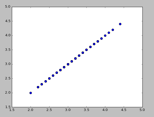
import matplotlib.pyplot as plt
plt.scatter(x,x,s=50,cmap="rainbow");
plt.show()
运行结果:
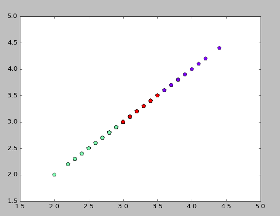
2. 鸢尾花花瓣长度数据做聚类并用散点图显示
import numpy as np
from sklearn.datasets import load_iris

iris = load_iris()
x = iris.data[:, 1]
y = np.zeros(150)

def initcent(x, k):  # 初始聚类中心数组
    return x[0:k].reshape(k)

def nearest(kc, i):  # 数组中的值,与聚类中心最小距离所在类别的索引号
    d = (abs(kc - i))
    w = np.where(d == np.min(d))
    return w[0][0]

def kcmean(x, y, kc, k):  # 计算各聚类新均值
    l = list(kc)
    flag = False
    for c in range(k):
        m = np.where(y == c)
        n = np.mean(x[m])
        if l[c] != n:
            l[c] = n
            flag = True  # 聚类中心发生变化
    return (np.array(l), flag)

def xclassify(x, y, kc):
    for i in range(x.shape[0]):  # 对数组的每个值分类
        y[i] = nearest(kc, x[i])
    return y
k = 3
kc = initcent(x, k)
flag = True
print(x, y, kc, flag)
while flag:
    y = xclassify(x, y, kc)
    kc, flag = kcmean(x, y, kc, k)
print(y, kc, type(kc))

import matplotlib.pyplot as plt
plt.scatter(x,x,c=y,s=50,cmap='rainbow',marker='p',alpha=1.5);
plt.show()
运行结果:
[3.5 3.  3.2 3.1 3.6 3.9 3.4 3.4 2.9 3.1 3.7 3.4 3.  3.  4.  4.4 3.9 3.5
 3.8 3.8 3.4 3.7 3.6 3.3 3.4 3.  3.4 3.5 3.4 3.2 3.1 3.4 4.1 4.2 3.1 3.2
 3.5 3.1 3.  3.4 3.5 2.3 3.2 3.5 3.8 3.  3.8 3.2 3.7 3.3 3.2 3.2 3.1 2.3
 2.8 2.8 3.3 2.4 2.9 2.7 2.  3.  2.2 2.9 2.9 3.1 3.  2.7 2.2 2.5 3.2 2.8
 2.5 2.8 2.9 3.  2.8 3.  2.9 2.6 2.4 2.4 2.7 2.7 3.  3.4 3.1 2.3 3.  2.5
 2.6 3.  2.6 2.3 2.7 3.  2.9 2.9 2.5 2.8 3.3 2.7 3.  2.9 3.  3.  2.5 2.9
 2.5 3.6 3.2 2.7 3.  2.5 2.8 3.2 3.  3.8 2.6 2.2 3.2 2.8 2.8 2.7 3.3 3.2
 2.8 3.  2.8 3.  2.8 3.8 2.8 2.8 2.6 3.  3.4 3.1 3.  3.1 3.1 3.1 2.7 3.2
 3.3 3.  2.5 3.  3.4 3. ] [0. 0. 0. 0. 0. 0. 0. 0. 0. 0. 0. 0. 0. 0. 0. 0. 0. 0. 0. 0. 0. 0. 0. 0.
 0. 0. 0. 0. 0. 0. 0. 0. 0. 0. 0. 0. 0. 0. 0. 0. 0. 0. 0. 0. 0. 0. 0. 0.
 0. 0. 0. 0. 0. 0. 0. 0. 0. 0. 0. 0. 0. 0. 0. 0. 0. 0. 0. 0. 0. 0. 0. 0.
 0. 0. 0. 0. 0. 0. 0. 0. 0. 0. 0. 0. 0. 0. 0. 0. 0. 0. 0. 0. 0. 0. 0. 0.
 0. 0. 0. 0. 0. 0. 0. 0. 0. 0. 0. 0. 0. 0. 0. 0. 0. 0. 0. 0. 0. 0. 0. 0.
 0. 0. 0. 0. 0. 0. 0. 0. 0. 0. 0. 0. 0. 0. 0. 0. 0. 0. 0. 0. 0. 0. 0. 0.
 0. 0. 0. 0. 0. 0.] [3.5 3.  3.2] True
[2. 2. 2. 2. 0. 0. 2. 2. 1. 2. 0. 2. 2. 2. 0. 0. 0. 2. 0. 0. 2. 0. 0. 2.
 2. 2. 2. 2. 2. 2. 2. 2. 0. 0. 2. 2. 2. 2. 2. 2. 2. 1. 2. 2. 0. 2. 0. 2.
 0. 2. 2. 2. 2. 1. 1. 1. 2. 1. 1. 1. 1. 2. 1. 1. 1. 2. 2. 1. 1. 1. 2. 1.
 1. 1. 1. 2. 1. 2. 1. 1. 1. 1. 1. 1. 2. 2. 2. 1. 2. 1. 1. 2. 1. 1. 1. 2.
 1. 1. 1. 1. 2. 1. 2. 1. 2. 2. 1. 1. 1. 0. 2. 1. 2. 1. 1. 2. 2. 0. 1. 1.
 2. 1. 1. 1. 2. 2. 1. 2. 1. 2. 1. 0. 1. 1. 1. 2. 2. 2. 2. 2. 2. 2. 1. 2.
 2. 2. 1. 2. 2. 2.] [3.84444444 2.64035088 3.17866667] <class 'numpy.ndarray'>
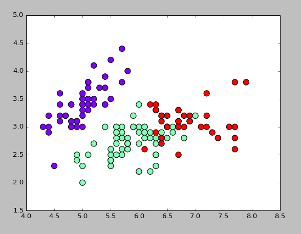
3. 用sklearn.cluster.KMeans,鸢尾花花瓣长度数据做聚类并用散点图显示.
import matplotlib.pyplot as plt
import numpy as np
from sklearn.datasets import load_iris
iris=load_iris()
X=iris.data
print(X)
from sklearn.cluster import KMeans
est=KMeans(n_clusters=3)
est.fit(X)
kc=est.cluster_centers_
y_kmeans=est.predict(X)
print(y_kmeans,kc)
print(kc.shape,y_kmeans.shape,X.shape)
plt.scatter(X[:,0],X[:,1],c=y_kmeans,s=100,cmap='rainbow');
plt.show()
运行结果:
[[5.1 3.5 1.4 0.2]
 [4.9 3.  1.4 0.2]
 [4.7 3.2 1.3 0.2]
 [4.6 3.1 1.5 0.2]
 [5.  3.6 1.4 0.2]
 [5.4 3.9 1.7 0.4]
 [4.6 3.4 1.4 0.3]
 [5.  3.4 1.5 0.2]
 [4.4 2.9 1.4 0.2]
 [4.9 3.1 1.5 0.1]
 [5.4 3.7 1.5 0.2]
 [4.8 3.4 1.6 0.2]
 [4.8 3.  1.4 0.1]
 [4.3 3.  1.1 0.1]
 [5.8 4.  1.2 0.2]
 [5.7 4.4 1.5 0.4]
 [5.4 3.9 1.3 0.4]
 [5.1 3.5 1.4 0.3]
 [5.7 3.8 1.7 0.3]
 [5.1 3.8 1.5 0.3]
 [5.4 3.4 1.7 0.2]
 [5.1 3.7 1.5 0.4]
 [4.6 3.6 1.  0.2]
 [5.1 3.3 1.7 0.5]
 [4.8 3.4 1.9 0.2]
 [5.  3.  1.6 0.2]
 [5.  3.4 1.6 0.4]
 [5.2 3.5 1.5 0.2]
 [5.2 3.4 1.4 0.2]
 [4.7 3.2 1.6 0.2]
 [4.8 3.1 1.6 0.2]
 [5.4 3.4 1.5 0.4]
 [5.2 4.1 1.5 0.1]
 [5.5 4.2 1.4 0.2]
 [4.9 3.1 1.5 0.1]
 [5.  3.2 1.2 0.2]
 [5.5 3.5 1.3 0.2]
 [4.9 3.1 1.5 0.1]
 [4.4 3.  1.3 0.2]
 [5.1 3.4 1.5 0.2]
 [5.  3.5 1.3 0.3]
 [4.5 2.3 1.3 0.3]
 [4.4 3.2 1.3 0.2]
 [5.  3.5 1.6 0.6]
 [5.1 3.8 1.9 0.4]
 [4.8 3.  1.4 0.3]
 [5.1 3.8 1.6 0.2]
 [4.6 3.2 1.4 0.2]
 [5.3 3.7 1.5 0.2]
 [5.  3.3 1.4 0.2]
 [7.  3.2 4.7 1.4]
 [6.4 3.2 4.5 1.5]
 [6.9 3.1 4.9 1.5]
 [5.5 2.3 4.  1.3]
 [6.5 2.8 4.6 1.5]
 [5.7 2.8 4.5 1.3]
 [6.3 3.3 4.7 1.6]
 [4.9 2.4 3.3 1. ]
 [6.6 2.9 4.6 1.3]
 [5.2 2.7 3.9 1.4]
 [5.  2.  3.5 1. ]
 [5.9 3.  4.2 1.5]
 [6.  2.2 4.  1. ]
 [6.1 2.9 4.7 1.4]
 [5.6 2.9 3.6 1.3]
 [6.7 3.1 4.4 1.4]
 [5.6 3.  4.5 1.5]
 [5.8 2.7 4.1 1. ]
 [6.2 2.2 4.5 1.5]
 [5.6 2.5 3.9 1.1]
 [5.9 3.2 4.8 1.8]
 [6.1 2.8 4.  1.3]
 [6.3 2.5 4.9 1.5]
 [6.1 2.8 4.7 1.2]
 [6.4 2.9 4.3 1.3]
 [6.6 3.  4.4 1.4]
 [6.8 2.8 4.8 1.4]
 [6.7 3.  5.  1.7]
 [6.  2.9 4.5 1.5]
 [5.7 2.6 3.5 1. ]
 [5.5 2.4 3.8 1.1]
 [5.5 2.4 3.7 1. ]
 [5.8 2.7 3.9 1.2]
 [6.  2.7 5.1 1.6]
 [5.4 3.  4.5 1.5]
 [6.  3.4 4.5 1.6]
 [6.7 3.1 4.7 1.5]
 [6.3 2.3 4.4 1.3]
 [5.6 3.  4.1 1.3]
 [5.5 2.5 4.  1.3]
 [5.5 2.6 4.4 1.2]
 [6.1 3.  4.6 1.4]
 [5.8 2.6 4.  1.2]
 [5.  2.3 3.3 1. ]
 [5.6 2.7 4.2 1.3]
 [5.7 3.  4.2 1.2]
 [5.7 2.9 4.2 1.3]
 [6.2 2.9 4.3 1.3]
 [5.1 2.5 3.  1.1]
 [5.7 2.8 4.1 1.3]
 [6.3 3.3 6.  2.5]
 [5.8 2.7 5.1 1.9]
 [7.1 3.  5.9 2.1]
 [6.3 2.9 5.6 1.8]
 [6.5 3.  5.8 2.2]
 [7.6 3.  6.6 2.1]
 [4.9 2.5 4.5 1.7]
 [7.3 2.9 6.3 1.8]
 [6.7 2.5 5.8 1.8]
 [7.2 3.6 6.1 2.5]
 [6.5 3.2 5.1 2. ]
 [6.4 2.7 5.3 1.9]
 [6.8 3.  5.5 2.1]
 [5.7 2.5 5.  2. ]
 [5.8 2.8 5.1 2.4]
 [6.4 3.2 5.3 2.3]
 [6.5 3.  5.5 1.8]
 [7.7 3.8 6.7 2.2]
 [7.7 2.6 6.9 2.3]
 [6.  2.2 5.  1.5]
 [6.9 3.2 5.7 2.3]
 [5.6 2.8 4.9 2. ]
 [7.7 2.8 6.7 2. ]
 [6.3 2.7 4.9 1.8]
 [6.7 3.3 5.7 2.1]
 [7.2 3.2 6.  1.8]
 [6.2 2.8 4.8 1.8]
 [6.1 3.  4.9 1.8]
 [6.4 2.8 5.6 2.1]
 [7.2 3.  5.8 1.6]
 [7.4 2.8 6.1 1.9]
 [7.9 3.8 6.4 2. ]
 [6.4 2.8 5.6 2.2]
 [6.3 2.8 5.1 1.5]
 [6.1 2.6 5.6 1.4]
 [7.7 3.  6.1 2.3]
 [6.3 3.4 5.6 2.4]
 [6.4 3.1 5.5 1.8]
 [6.  3.  4.8 1.8]
 [6.9 3.1 5.4 2.1]
 [6.7 3.1 5.6 2.4]
 [6.9 3.1 5.1 2.3]
 [5.8 2.7 5.1 1.9]
 [6.8 3.2 5.9 2.3]
 [6.7 3.3 5.7 2.5]
 [6.7 3.  5.2 2.3]
 [6.3 2.5 5.  1.9]
 [6.5 3.  5.2 2. ]
 [6.2 3.4 5.4 2.3]
 [5.9 3.  5.1 1.8]]
[0 0 0 0 0 0 0 0 0 0 0 0 0 0 0 0 0 0 0 0 0 0 0 0 0 0 0 0 0 0 0 0 0 0 0 0 0
 0 0 0 0 0 0 0 0 0 0 0 0 0 1 1 2 1 1 1 1 1 1 1 1 1 1 1 1 1 1 1 1 1 1 1 1 1
 1 1 1 2 1 1 1 1 1 1 1 1 1 1 1 1 1 1 1 1 1 1 1 1 1 1 2 1 2 2 2 2 1 2 2 2 2
 2 2 1 1 2 2 2 2 1 2 1 2 1 2 2 1 1 2 2 2 2 2 1 2 2 2 2 1 2 2 2 1 2 2 2 1 2
 2 1] [[5.006      3.418      1.464      0.244     ]
 [5.9016129  2.7483871  4.39354839 1.43387097]
 [6.85       3.07368421 5.74210526 2.07105263]]
(3, 4) (150,) (150, 4)
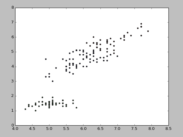
4. 鸢尾花完整数据做聚类并用散点图显示
from sklearn.cluster import KMeans
import numpy as np
from sklearn.datasets import load_iris
import matplotlib.pyplot as plt
data = load_iris()
iris = data.data
petal_len = iris
print(petal_len)
k_means = KMeans(n_clusters=3) #三个聚类中心
result = k_means.fit(petal_len) #Kmeans自动分类
kc = result.cluster_centers_ #自动分类后的聚类中心
y_means = k_means.predict(petal_len) #预测Y值
plt.scatter(petal_len[:,0],petal_len[:,2],c=y_means, marker='*', label='see')
plt.show()
运行结果:
from sklearn.cluster import KMeans
import numpy as np
from sklearn.datasets import load_iris
import matplotlib.pyplot as plt
data = load_iris()
iris = data.data
petal_len = iris
print(petal_len)
k_means = KMeans(n_clusters=3) #三个聚类中心
result = k_means.fit(petal_len) #Kmeans自动分类
kc = result.cluster_centers_ #自动分类后的聚类中心
y_means = k_means.predict(petal_len) #预测Y值
plt.scatter(petal_len[:,0],petal_len[:,2],c=y_means, marker='*', label='see')
plt.show()

 浙公网安备 33010602011771号