Tensorflow--Matplotlib

代码：

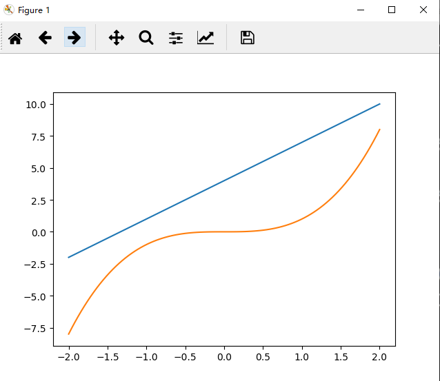
# -*- coding: UTF-8 -*-

# 引入 Matplotlib 的分模块 pyplot
import matplotlib.pyplot as plt
# 引入 numpy
import numpy as np

# 创建数据
x = np.linspace(-2, 2, 100) #在一定范围内生成一系列点线
# y = 3 * x + 4
y1 = 3 * x + 4
y2 = x ** 3

# 创建图像
# plt.plot(x, y)
plt.plot(x, y1)
plt.plot(x, y2)

# 显示图像
plt.show()

运行结果：

代码：

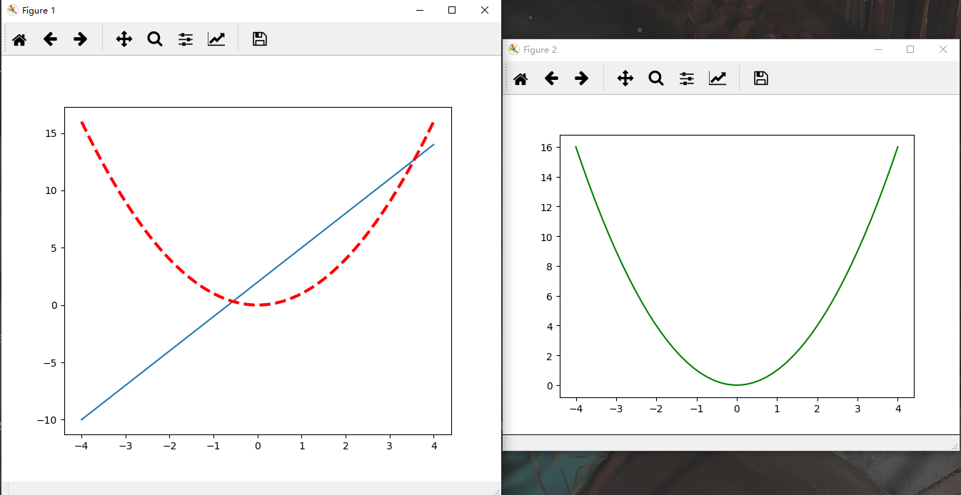
# -*- coding: UTF-8 -*-

import matplotlib.pyplot as plt
import numpy as np

# 创建数据
x = np.linspace(-4, 4, 50)
y1 = 3 * x + 2
y2 = x ** 2

# 第一张图
plt.figure(num=1, figsize=(7, 6))
plt.plot(x, y1)
plt.plot(x, y2, color="red", linewidth=3.0, linestyle="--")

# 第二张图
plt.figure(num=2)
plt.plot(x, y2, color="green")

# 显示所有图像
plt.show()

运行结果：

 代码：

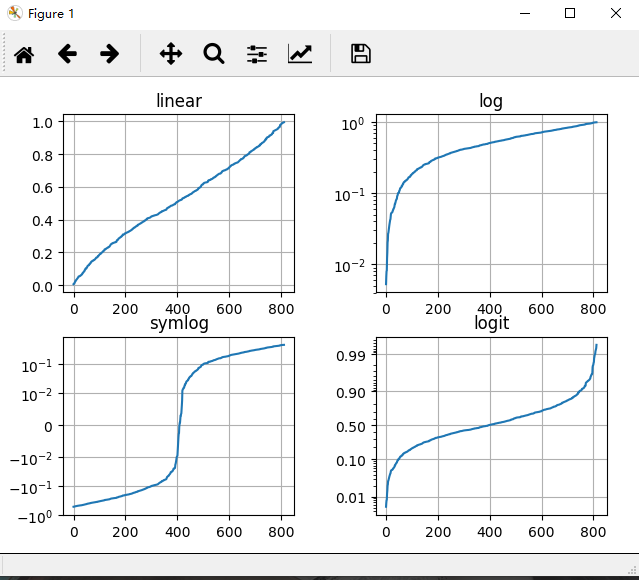
# -*- coding: UTF-8 -*-

import numpy as np
import matplotlib.pyplot as plt

from matplotlib.ticker import NullFormatter

"""
多个子图
"""

# 为了能够复现
np.random.seed(1)

y = np.random.normal(loc=0.5, scale=0.4, size=1000)
y = y[(y > 0) & (y < 1)]
y.sort()
x = np.arange(len(y))

plt.figure(1)

# linear
plt.subplot(221)
plt.plot(x, y)
plt.yscale('linear')
plt.title('linear')
plt.grid(True)

# log
plt.subplot(222)
plt.plot(x, y)
plt.yscale('log')
plt.title('log')
plt.grid(True)

# symmetric log
plt.subplot(223)
plt.plot(x, y - y.mean())
plt.yscale('symlog', linthreshy=0.01)
plt.title('symlog')
plt.grid(True)

# logit
plt.subplot(224)
plt.plot(x, y)
plt.yscale('logit')
plt.title('logit')
plt.grid(True)
plt.gca().yaxis.set_minor_formatter(NullFormatter())
plt.subplots_adjust(top=0.92, bottom=0.08, left=0.10, right=0.95, hspace=0.25,
                    wspace=0.35)

plt.show()

运行结果：

 代码：

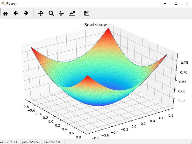
# -*- coding: UTF-8 -*-

import matplotlib.pyplot as plt
from mpl_toolkits.mplot3d import Axes3D
import numpy as np

"""
碗状图形
"""

fig = plt.figure(figsize=(8, 5))
ax1 = Axes3D(fig)

alpha = 0.8
r = np.linspace(-alpha, alpha, 100)
X, Y = np.meshgrid(r, r)
l = 1. / (1 + np.exp(-(X ** 2 + Y ** 2)))

ax1.plot_wireframe(X, Y, l)
ax1.plot_surface(X, Y, l, cmap=plt.get_cmap("rainbow"))  # 彩虹配色
ax1.set_title("Bowl shape")

plt.show()

运行结果：

 代码：

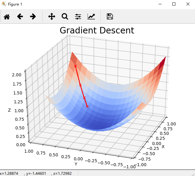
# -*- coding: UTF-8 -*-

"""
Gradient Descent 的 3D 动态图示
"""

import numpy as np
from matplotlib import cm
import matplotlib.pyplot as plt
import mpl_toolkits.mplot3d.axes3d as p3
import matplotlib.animation as animation


nb_steps = 20
x0 = np.array([0.8, 0.8])
learning_rate = 0.1


def cost_function(x):
    return x[0]**2 + x[1]**2


def gradient_cost_function(x):
    return np.array([2*x[0], 2*x[1]])


def gen_line():
    x = x0.copy()
    data = np.empty((3, nb_steps+1))
    data[:, 0] = np.concatenate((x, [cost_function(x)]))
    for t in range(1, nb_steps+1):
        grad = gradient_cost_function(x)
        x -= learning_rate * grad
        data[:, t] = np.concatenate((x, [cost_function(x)]))
    return data


def update_line(num, data, line):
    line.set_data(data[:2, :num])
    line.set_3d_properties(data[2, :num])
    return line


fig = plt.figure()
fig.suptitle("Gradient Descent", fontsize=20)
ax = p3.Axes3D(fig)

X = np.arange(-0.5, 1, 0.1)
Y = np.arange(-1, 1, 0.1)
X, Y = np.meshgrid(X, Y)
Z = cost_function((X, Y))

surf = ax.plot_surface(X, Y, Z, rstride=1, cstride=1, cmap=cm.coolwarm, linewidth=0, antialiased=False)

data = gen_line()

line = ax.plot(data[0, 0:1], data[0, 0:1], data[0, 0:1], 'rx-', linewidth=2)[0]

ax.view_init(30, -160)

ax.set_xlim3d([-1.0, 1.0])
ax.set_xlabel('X')

ax.set_ylim3d([-1.0, 1.0])
ax.set_ylabel('Y')

ax.set_zlim3d([0.0, 2.0])
ax.set_zlabel('Z')

line_ani = animation.FuncAnimation(fig, update_line, nb_steps+1, fargs=(data, line), interval=200, blit=False)

line_ani.save('gradient_descent.gif', dpi=80, writer='imagemagick')

plt.show()

运行结果：