
作业05
1.本节重点知识点用自己的话总结出来,可以配上图片,以及说明该知识点的重要性
网课上讲的知识点老重要了,那可全都是重点啊。
回归算法的定义:我们可以根据现有提供的数据进行运算,构建函数模型,对数据进行训练,从而可以用构建好的模型进行预测,得出的结果可以有离散型和连续型。
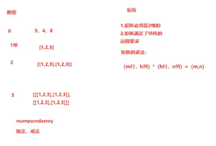
矩阵:矩阵一个按照长方阵列排列的复数或实数集合,我们可以应用矩阵进行乘法应算、减法应算和乘法应算等等。
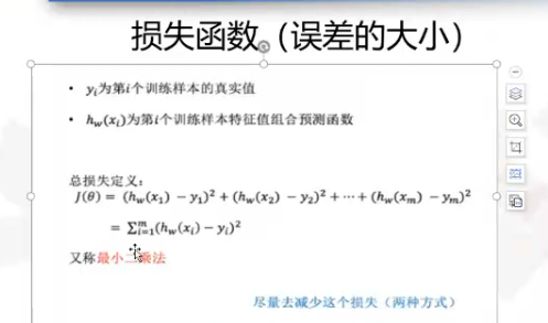
损失函数:通过函数模型运算得到的结果于实际结果的误差大小值,其值是非负数的。
2.思考线性回归算法可以用来做什么?(大家尽量不要写重复)
可以用来检测混凝土质量,来源:https://www.ibm.com/developerworks/cn/analytics/library/ba-lo-machine-learning-cement-quality/index.html
3.自主编写线性回归算法 ,数据可以自己造,或者从网上获取。(加分题)
加分加分!!
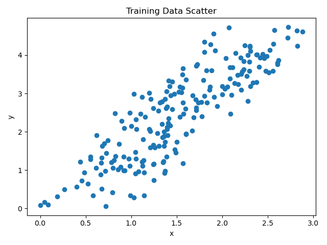
(1)生成数据
代码:
1 # Create the data
2 x = [(i+random.random()*100)/100 for i in range(200)]
3 y = [((2*i+1)+random.random()*100)/100 for i in range(200)]
4 plt.xlabel('x')
5 plt.ylabel('y')
6 plt.title('Training Data Scatter')
7 plt.scatter(x, y)
8 plt.show()
所生成数据的散点图:
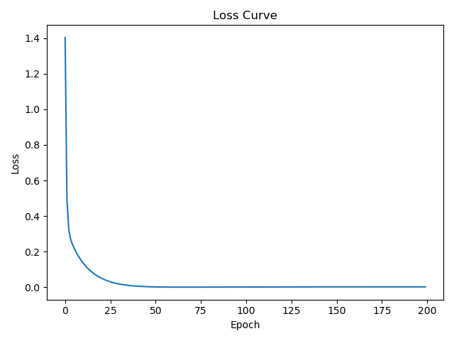
(2)使用线性回归算法进行训练,学习速率设置为0.001,获得w值与b值
代码:
 1 # Train for w and b
 2 w = random.random()
 3 b = random.random()
 4 a1 = []
 5 b1 = []
 6 loss = None
 7 for i in range(200):
 8     for x1, y1 in zip(x, y):
 9         y_pre = w*x1+b # Prediction
10         bias = (y_pre-y1) # Bias
11         loss = bias**2 # Loss
12         dw = 2*bias*x1 # Differentiate of w
13         db = 2*bias*1 # Differentiate of b
14         w = w-0.001*dw # Set learning rate to 0.001
15         b = b-0.001*db # Set learning rate to 0.001
16         print('loss={0},w={1},b={2}'. format(loss, w, b))
17     a1.append(i)
18     b1.append(loss)
19 plt.xlabel('Epoch')
20 plt.ylabel('Loss')
21 plt.title('Loss Curve')
22 plt.plot(a1, b1)
23 plt.show()
24 print('w: {}\nb: {}'.format(w, b)) # Print result
200轮后所得w值与b值:

200轮后的Loss曲线:
(3)使用训练结果进行预测,并画出线性回归曲线
代码:
1 # Predict
2 y_pred = [w*i+b for i in x] # Get predictions
3 plt.plot(x, y_pred) # Linear Regression line
4 plt.xlabel('x')
5 plt.ylabel('y')
6 plt.title('Linear Regression line')
7 plt.scatter(x, y, color='red')
8 plt.show()
样本散点图与线性回归曲线:

完整代码:
 1 import random
 2 import matplotlib.pyplot as plt
 3
 4 # Create the data
 5 x = [(i+random.random()*100)/100 for i in range(200)]
 6 y = [((2*i+1)+random.random()*100)/100 for i in range(200)]
 7 plt.xlabel('x')
 8 plt.ylabel('y')
 9 plt.title('Training Data Scatter')
10 plt.scatter(x, y)
11 plt.show()
12
13 # Train for w and b
14 w = random.random()
15 b = random.random()
16 a1 = []
17 b1 = []
18 loss = None
19 for i in range(200):
20     for x1, y1 in zip(x, y):
21         y_pre = w*x1+b # Prediction
22         bias = (y_pre-y1) # Bias
23         loss = bias**2 # Loss
24         dw = 2*bias*x1 # Differentiate of w
25         db = 2*bias*1 # Differentiate of b
26         w = w-0.001*dw # Set learning rate to 0.001
27         b = b-0.001*db # Set learning rate to 0.001
28         print('loss={0},w={1},b={2}'. format(loss, w, b))
29     a1.append(i)
30     b1.append(loss)
31 plt.xlabel('Epoch')
32 plt.ylabel('Loss')
33 plt.title('Loss Curve')
34 plt.plot(a1, b1)
35 plt.show()
36 print('w: {}\nb: {}'.format(w, b)) # Print result
37
38 # Predict
39 y_pred = [w*i+b for i in x] # Get predictions
40 plt.plot(x, y_pred) # Linear Regression line
41 plt.xlabel('x')
42 plt.ylabel('y')
43 plt.title('Linear Regression line')
44 plt.scatter(x, y, color='red')
45 plt.show()