

《python深度学习》笔记---5.4-3、卷积网络可视化-热力图
《python深度学习》笔记---5.4-3、卷积网络可视化-热力图
一、总结
一句话总结:
【一张图像的哪一部分让卷积神经网络做出了最终的分类决策】:可视化类激活的热力图,它有助于了解一张图像的哪一部分让卷积神经网络做出了 最终的分类决策。这有助于对卷积神经网络的决策过程进行调试,特别是出现分类错误的情况下。 这种方法还可以定位图像中的特定目标。
【类激活图】:这种通用的技术叫作类激活图(CAM,class activation map)可视化,它是指对输入图像生 成类激活的热力图。
【每个位置对该类别的重要程度】:类激活热力图是与特定输出类别相关的二维分数网格,对任何输入图像的 每个位置都要进行计算,它表示每个位置对该类别的重要程度。
1、类激活的热力图解决本实例中的问题?
网络为什么会认为这张图像中包含一头非洲象?
非洲象在图像中的什么位置?
二、5.4-3、卷积网络可视化-热力图
博客对应课程的视频位置:
Visualizing heatmaps of class activation
We will introduce one more visualization technique, one that is useful for understanding which parts of a given image led a convnet to its final classification decision. This is helpful for "debugging" the decision process of a convnet, in particular in case of a classification mistake. It also allows you to locate specific objects in an image.
This general category of techniques is called "Class Activation Map" (CAM) visualization, and consists in producing heatmaps of "class activation" over input images. A "class activation" heatmap is a 2D grid of scores associated with an specific output class, computed for every location in any input image, indicating how important each location is with respect to the class considered. For instance, given a image fed into one of our "cat vs. dog" convnet, Class Activation Map visualization allows us to generate a heatmap for the class "cat", indicating how cat-like different parts of the image are, and likewise for the class "dog", indicating how dog-like differents parts of the image are.
The specific implementation we will use is the one described in Grad-CAM: Why did you say that? Visual Explanations from Deep Networks via Gradient-based Localization. It is very simple: it consists in taking the output feature map of a convolution layer given an input image, and weighing every channel in that feature map by the gradient of the class with respect to the channel. Intuitively, one way to understand this trick is that we are weighting a spatial map of "how intensely the input image activates different channels" by "how important each channel is with regard to the class", resulting in a spatial map of "how intensely the input image activates the class".
We will demonstrate this technique using the pre-trained VGG16 network again:
from keras.applications.vgg16 import VGG16

K.clear_session()

# Note that we are including the densely-connected classifier on top;
# all previous times, we were discarding it.
model = VGG16(weights='imagenet')
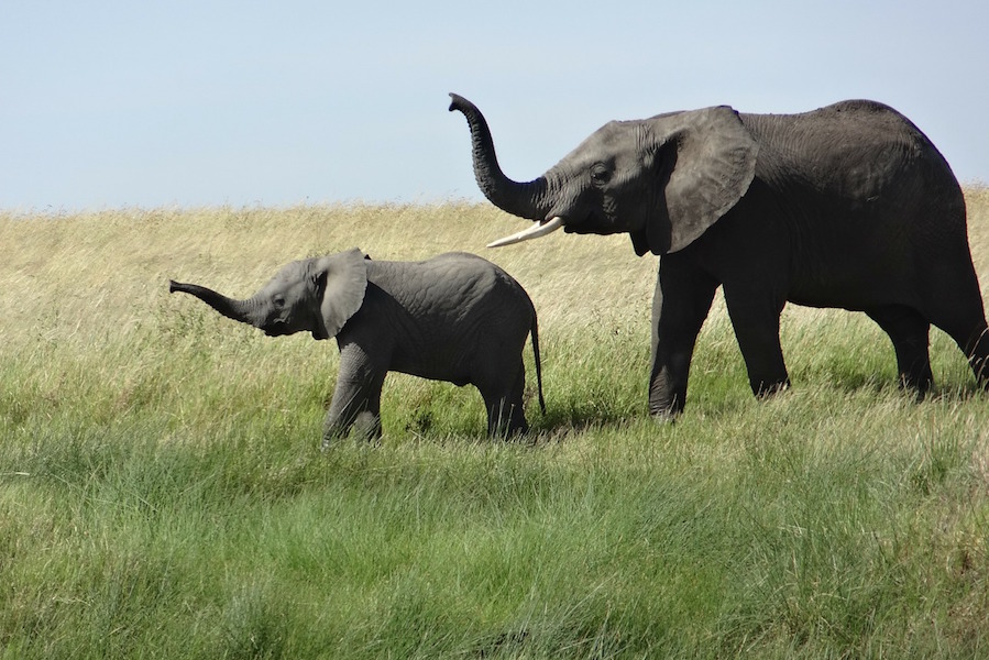
Let's consider the following image of two African elephants, possible a mother and its cub, strolling in the savanna (under a Creative Commons license):
Let's convert this image into something the VGG16 model can read: the model was trained on images of size 224x244, preprocessed according to a few rules that are packaged in the utility function keras.applications.vgg16.preprocess_input. So we need to load the image, resize it to 224x224, convert it to a Numpy float32 tensor, and apply these pre-processing rules.
from keras.preprocessing import image
from keras.applications.vgg16 import preprocess_input, decode_predictions
import numpy as np

# The local path to our target image
img_path = '/Users/fchollet/Downloads/creative_commons_elephant.jpg'

# `img` is a PIL image of size 224x224
img = image.load_img(img_path, target_size=(224, 224))

# `x` is a float32 Numpy array of shape (224, 224, 3)
x = image.img_to_array(img)

# We add a dimension to transform our array into a "batch"
# of size (1, 224, 224, 3)
x = np.expand_dims(x, axis=0)

# Finally we preprocess the batch
# (this does channel-wise color normalization)
x = preprocess_input(x)
preds = model.predict(x)
print('Predicted:', decode_predictions(preds, top=3)[0])
The top-3 classes predicted for this image are:
- African elephant (with 92.5% probability)
- Tusker (with 7% probability)
- Indian elephant (with 0.4% probability)
Thus our network has recognized our image as containing an undetermined quantity of African elephants. The entry in the prediction vector that was maximally activated is the one corresponding to the "African elephant" class, at index 386:
np.argmax(preds[0])
To visualize which parts of our image were the most "African elephant"-like, let's set up the Grad-CAM process:
# This is the "african elephant" entry in the prediction vector
african_elephant_output = model.output[:, 386]

# The is the output feature map of the `block5_conv3` layer,
# the last convolutional layer in VGG16
last_conv_layer = model.get_layer('block5_conv3')

# This is the gradient of the "african elephant" class with regard to
# the output feature map of `block5_conv3`
grads = K.gradients(african_elephant_output, last_conv_layer.output)[0]

# This is a vector of shape (512,), where each entry
# is the mean intensity of the gradient over a specific feature map channel
pooled_grads = K.mean(grads, axis=(0, 1, 2))

# This function allows us to access the values of the quantities we just defined:
# `pooled_grads` and the output feature map of `block5_conv3`,
# given a sample image
iterate = K.function([model.input], [pooled_grads, last_conv_layer.output[0]])

# These are the values of these two quantities, as Numpy arrays,
# given our sample image of two elephants
pooled_grads_value, conv_layer_output_value = iterate([x])

# We multiply each channel in the feature map array
# by "how important this channel is" with regard to the elephant class
for i in range(512):
    conv_layer_output_value[:, :, i] *= pooled_grads_value[i]

# The channel-wise mean of the resulting feature map
# is our heatmap of class activation
heatmap = np.mean(conv_layer_output_value, axis=-1)
For visualization purpose, we will also normalize the heatmap between 0 and 1:
heatmap = np.maximum(heatmap, 0)
heatmap /= np.max(heatmap)
plt.matshow(heatmap)
plt.show()

Finally, we will use OpenCV to generate an image that superimposes the original image with the heatmap we just obtained:
import cv2

# We use cv2 to load the original image
img = cv2.imread(img_path)

# We resize the heatmap to have the same size as the original image
heatmap = cv2.resize(heatmap, (img.shape[1], img.shape[0]))

# We convert the heatmap to RGB
heatmap = np.uint8(255 * heatmap)

# We apply the heatmap to the original image
heatmap = cv2.applyColorMap(heatmap, cv2.COLORMAP_JET)

# 0.4 here is a heatmap intensity factor
superimposed_img = heatmap * 0.4 + img

# Save the image to disk
cv2.imwrite('/Users/fchollet/Downloads/elephant_cam.jpg', superimposed_img)

This visualisation technique answers two important questions:
- Why did the network think this image contained an African elephant?
- Where is the African elephant located in the picture?
In particular, it is interesting to note that the ears of the elephant cub are strongly activated: this is probably how the network can tell the difference between African and Indian elephants.

 浙公网安备 33010602011771号