tensorflow2知识总结---1、线性回归实例

tensorflow2知识总结---1、线性回归实例

一、总结

一句话总结：

第一步：创建模型：model = tf.keras.Sequential() 后面用model的add方法添加layers就好

第二步：训练模型：history = model.fit(x,y,epochs=5000)

第三步：用训练好的模型做预测：y1 = model.predict(x)

第一步：创建模型
#4.tf.keras实现线性回归
x = data.Education
y = data.Income
# 顺序模型
model = tf.keras.Sequential()
# 添加dense层
model.add(tf.keras.layers.Dense(1,input_shape=(1,)))
# ax+b
model.summary()


第二步：训练模型
# 优化算法 梯度下降adam，学习速率使用的是默认的  
# MSE均方误差
model.compile(optimizer='adam',loss='mse')
history = model.fit(x,y,epochs=5000) #epochs表示训练的次数


第三步：用训练好的模型做预测
y1 = model.predict(x)
# 预测20年教育的收入
model.predict(pd.Series([20]))

 

 

1、pandas读取csv文件？

data = pd.read_csv('./dataset/income.csv')

 

2、matplotlib画散点图？

plt.scatter(data.Education,data.Income)

import matplotlib.pyplot as plt
%matplotlib inline
plt.scatter(data.Education,data.Income)

 

 

3、tensorflow2创建线性回归模型（创建模型过程）？

a、顺序模型：model = tf.keras.Sequential()

b、添加dense层：model.add(tf.keras.layers.Dense(1,input_shape=(1,)))

c、模型概况（比如每层网络有多少待求参数）：model.summary()

 

 

4、模型添加时候model.add(tf.keras.layers.Dense(1,input_shape=(1,))) 是什么意思？

Dense(1,input_shape=(1,))中的前一个1表示一个神经元，input_shape中的1表示输入数据是1维

 

5、线性回归函数和神经网络的关系？

线性回归函数可以看做单个神经元

 

6、tensorflow2线性回归模型 训练模型过程？

A、设定优化算法：model.compile(optimizer='adam',loss='mse')

B、训练过程：history = model.fit(x,y,epochs=5000)

# 优化算法 梯度下降adam，学习速率使用的是默认的  
# MSE均方误差
model.compile(optimizer='adam',loss='mse')
history = model.fit(x,y,epochs=5000) #epochs表示训练的次数

 

 

7、tensorflow2线性回归模型 预测过程？

model对象的predict方法：y1 = model.predict(x)

# 预测20年教育的收入
model.predict(pd.Series([20]))

 

 

 

二、线性回归实例

博客对应课程的视频位置：

 

In [35]:

 

 

import pandas as pd

data = pd.read_csv('./dataset/income.csv')

data

Out[35]:

	Unnamed: 0	Education	Income
0	1	10.000000	26.658839
1	2	10.401338	27.306435
2	3	10.842809	22.132410
3	4	11.244147	21.169841
4	5	11.645449	15.192634
5	6	12.086957	26.398951
6	7	12.048829	17.435307
7	8	12.889632	25.507885
8	9	13.290970	36.884595
9	10	13.732441	39.666109
10	11	14.133779	34.396281
11	12	14.635117	41.497994
12	13	14.978589	44.981575
13	14	15.377926	47.039595
14	15	15.779264	48.252578
15	16	16.220736	57.034251
16	17	16.622074	51.490919
17	18	17.023411	51.336621
18	19	17.464883	57.681998
19	20	17.866221	68.553714
20	21	18.267559	64.310925
21	22	18.709030	68.959009
22	23	19.110368	74.614639
23	24	19.511706	71.867195
24	25	19.913043	76.098135
25	26	20.354515	75.775216
26	27	20.755853	72.486055
27	28	21.167191	77.355021
28	29	21.598662	72.118790
29	30	22.000000	80.260571

In [36]:

 

 

import matplotlib.pyplot as plt

%matplotlib inline

plt.scatter(data.Education,data.Income)

​

Out[36]:

<matplotlib.collections.PathCollection at 0x1c3e1b3dac8>

找到合适的a和b，使得(f(x)-y)^2越小越好

In [37]:

 

#4.tf.keras实现线性回归

x = data.Education

y = data.Income

# 顺序模型

model = tf.keras.Sequential()

# 添加dense层

model.add(tf.keras.layers.Dense(1,input_shape=(1,)))

# ax+b

model.summary()

Model: "sequential_4"
_________________________________________________________________
Layer (type)                 Output Shape              Param #   
=================================================================
dense_3 (Dense)              (None, 1)                 2         
=================================================================
Total params: 2
Trainable params: 2
Non-trainable params: 0
_________________________________________________________________

(None, 1) 中的None是样本的维度

Param是两个，也就是a和b

In [39]:

 

# 优化算法 梯度下降adam，学习速率使用的是默认的  

# MSE均方误差

model.compile(optimizer='adam',loss='mse')

history = model.fit(x,y,epochs=5000) #epochs表示训练的次数

​

Epoch 1/5000
1/1 [==============================] - 0s 2ms/step - loss: 132.0959
Epoch 2/5000
1/1 [==============================] - 0s 0s/step - loss: 131.9527
Epoch 3/5000
......
Epoch 4999/5000
1/1 [==============================] - 0s 996us/step - loss: 95.0121
Epoch 5000/5000
1/1 [==============================] - 0s 0s/step - loss: 95.0086

In [40]:

 

# 预测x

y1 = model.predict(x)

y1

Out[40]:

array([[31.637905],
       [32.976357],
       [34.448647],
       [35.787098],
       [37.125427],
       [38.597843],
       [38.470688],
       [41.27474 ],
       [42.61319 ],
       [44.08548 ],
       [45.42393 ],
       [47.095875],
       [48.24135 ],
       [49.573124],
       [50.911575],
       [52.383865],
       [53.722317],
       [55.060764],
       [56.533062],
       [57.87151 ],
       [59.20996 ],
       [60.68225 ],
       [62.020702],
       [63.359146],
       [64.69759 ],
       [66.16989 ],
       [67.50835 ],
       [68.88014 ],
       [70.319084],
       [71.65753 ]], dtype=float32)

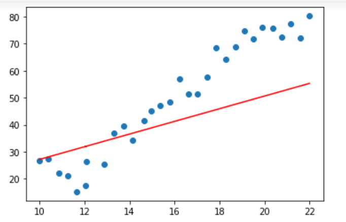
x = data.Education
y = data.Income
plt.scatter(x,y)

pred_y= w*x+b

plt.plot(x,pred_y,c='r')

 

 

 

 

线性回归函数可以看做单个神经元