
卷积神经网络预测Cifar10(Keras版本+PyTorch版本)
Keras版本
导入模块
from keras.datasets import cifar10
import numpy as np
from keras.utils import np_utils
import matplotlib.pyplot as plt
from keras.models import Sequential
from keras.layers import Dense,Dropout,Activation,Flatten,Conv2D,MaxPooling2D,ZeroPadding2D
import pandas as pd
np.random.seed(10)
加载并查看数据集
(x_Train,y_Train),(x_Test,y_Test) = cifar10.load_data()
print('train:',len(x_Train))
print('test:',len(x_Test))
print(x_Train.shape)
print(x_Train[0])
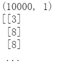
print(y_Test.shape)
print(y_Test)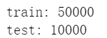
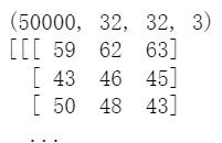
可以看到训练集有50000项,测试集有10000项
每个图像都是3维的,前两维度表示像素点,第三维度包含三个数,分别是红蓝绿通道。
定义工具类
label_dict={0:"airplane",
           1:"automobile",
           2:"bird",
           3:"cat",
           4:"deer",
           5:"dog",
           6:"frog",
           7:"horse",
           8:"ship",
           9:"truck"}
def plot_images_labels_prediction(images,labels,prediction,idx,num=10):
    fig = plt.gcf()
    fig.set_size_inches(12,14)
    if num>25 :
        num=25
    for i in range(0,num):
        ax=plt.subplot(5,5,i+1) #子图保存在ax中
        ax.imshow(images[idx+i],cmap='binary')
        title=str(i)+','+label_dict[ labels[i][0] ] #子图标签
        if(len(prediction)> 0):
            title+='=>'+label_dict[ prediction[i]] #如果有预测结果,就输出预测结果
        ax.set_title(title,fontsize=10)
        ax.set_xticks([]);
        ax.set_yticks([]);
    plt.show()
def show_train_history(history,train,validation):
    plt.plot(history.history[train])
    plt.plot(history.history[validation])
    plt.title('Train History')
    plt.xlabel('epoch')
    plt.ylabel(train)
    plt.legend(['train','validation'],loc='upper left')
    plt.show()
定义字典将标签和英文对应上
查看图像以及标签
plot_images_labels_prediction(x_Train,y_Train,[],0,25)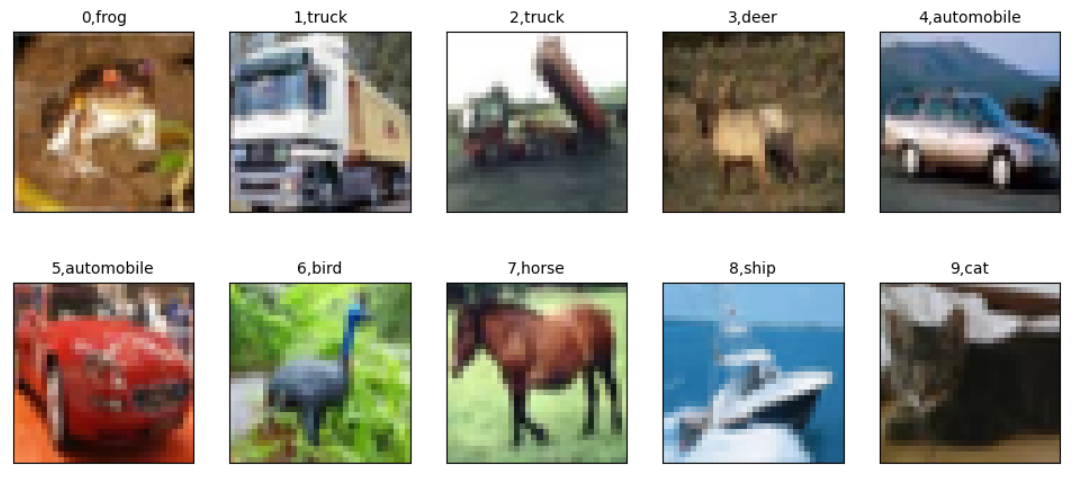 ........0号青蛙看着像是从游戏贴图里拔出来的🙄?!!!
数据预处理
x_Train_normalize=x_Train.astype('float32')/255.0 #归一化
x_Test_normalize=x_Test.astype('float32')/255.0
y_Train_OneHot=np_utils.to_categorical(y_Train) #转换为独热编码
y_Test_OneHot = np_utils.to_categorical(y_Test)
x_Train_normalize[0][0][0]
print(y_Train.shape)
print(y_Train_OneHot.shape)![]()
![]()
原本第二维只有一个数字,直接表示标签,转换成了10个数字,用0和1表示标签。
model=Sequential()
model.add(Conv2D(filters=32,             #卷积层1
                kernel_size=(3,3),
                input_shape=(32,32,3),
                activation='relu',
                padding='same'))
model.add(Dropout(rate=0.25))            #Dropout层1
model.add(MaxPooling2D(pool_size=(2,2))) #池化层1

model.add(Conv2D(filters=64,             #卷积层2
                kernel_size=(3,3),
                activation='relu',
                padding='same'))
model.add(Dropout(rate=0.25))            #Dropout层2
model.add(MaxPooling2D(pool_size=(2,2))) #池化层层2

model.add(Flatten())                     #平坦层
model.add(Dropout(rate=0.25))            #Dropout层3
model.add(Dense(units=1024,              #隐藏层
               activation='relu'))
model.add(Dropout(rate=0.25))            #输出层
model.add(Dense(units=10,activation='softmax'))
查看模型参数
print(model.summary())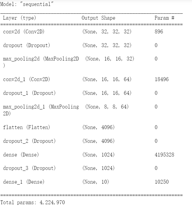
设置模型训练参数然后训练模型
model.compile(loss='categorical_crossentropy', #损失函数为交叉熵损失
optimizer='adam', #优化器选择adam
metrics=['accuracy']) #使用准确率为标准
train_history=model.fit(x=x_Train_normalize,
y=y_Train_OneHot,
validation_split=0.2,
epochs=10,
batch_size=128,
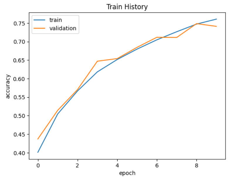
verbose=2)显示训练准确率和损失
show_train_history(train_history,'accuracy','val_accuracy')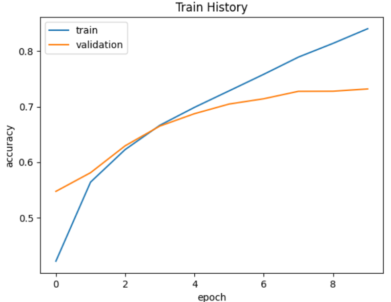
训练集上挺高,但是在验证集上最后却降低了,可能是过拟合了
show_train_history(train_history,'loss','val_loss')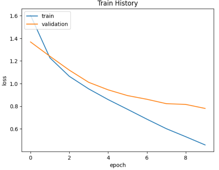
评估模型
scores=model.evaluate(x_Test_normalize,y_Test_OneHot,verbose=0)
scores[1]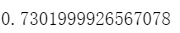
使用模型预测数据
prediction = model.predict(x_Test_normalize) #获取到的prediction每一项都包含十个浮点数,表示预测为各个类型的概率
prediction = np.argmax(prediction,axis=1) #每一项都取本项中十个浮点数最大的那个的下标,也就是标签
prediction[:10]![]()
显示图片和预测结果
plot_images_labels_prediction(x_Test,y_Test,prediction,idx=0)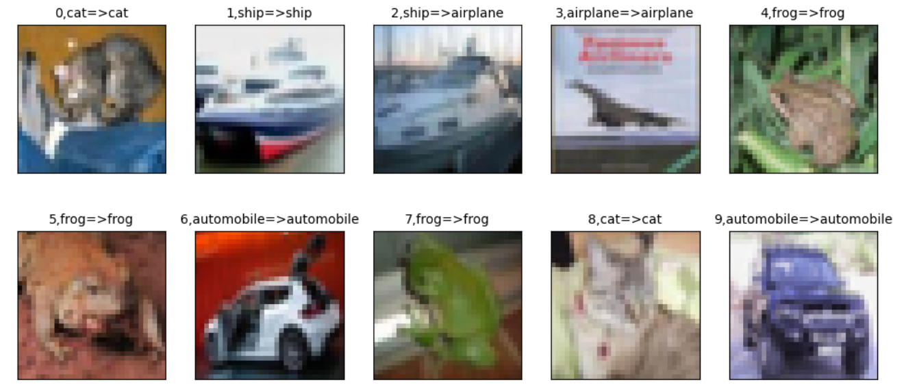
可以发现第三项应该是船,但是预测成了飞机。
显示一项的预测概率
Predicted_Probability = model.predict(x_Test_normalize)
def show_Predicted_Probability(y,prediction,x_img,Predicted_Probability,i):
    print('label:',label_dict[y[i][0]]),
    plt.figure(figsize=(2,2))
    plt.imshow(np.reshape(x_img[i],(32,32,3)))
    plt.show()
    for j in range(10): #输出每一个类型的预测结果
        print(label_dict[j]+' Probability:%1.9f'%(Predicted_Probability[i][j]))
show_Predicted_Probability(y_Test,prediction,x_Test,Predicted_Probability,2)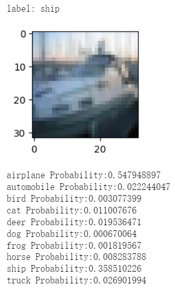
可以发现其中飞机的概率最高,但其实是船
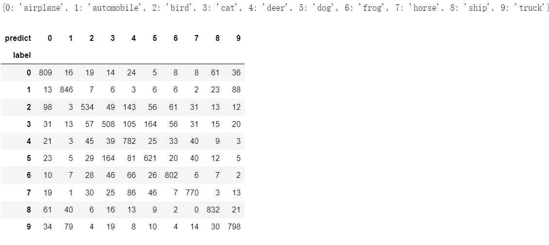
创建混淆矩阵
import pandas as pd
print(prediction.shape)  #输出预测集合的形状
print(y_Test.shape)      #输出测试集标签集的形状
y_Test_OneDim=y_Test.reshape(-1)   #将标签集合转为一位数组
print(y_Test_OneDim.shape)   #输出转换后标签集合的形状
print(label_dict)   #输出字典
pd.crosstab(y_Test_OneDim,prediction,rownames=['label'],colnames=['predict']) #创建混淆矩阵
因为原本标签集合是二维的,第二维只用一个数表示标签,而预测集合是一维的,要使两个集合匹配,然后创建混淆矩阵
![]()
3次的卷积运算神经网络
结构
model=Sequential()
model.add(Conv2D(filters=32,
                kernel_size=(3,3),
                input_shape=(32,32,3),
                activation='relu',
                padding='same'))
model.add(Dropout(rate=0.3))
model.add(Conv2D(filters=32,
                kernel_size=(3,3),
                activation='relu',
                padding='same'))
model.add(MaxPooling2D(pool_size=(2,2)))


model.add(Conv2D(filters=64,
                kernel_size=(3,3),
                activation='relu',
                padding='same'))
model.add(Dropout(rate=0.3))
model.add(Conv2D(filters=64,
                kernel_size=(3,3),
                activation='relu',
                padding='same'))
model.add(MaxPooling2D(pool_size=(2,2)))

model.add(Conv2D(filters=128,
                kernel_size=(3,3),
                activation='relu',
                padding='same'))
model.add(Dropout(rate=0.3))
model.add(Conv2D(filters=128,
                kernel_size=(3,3),
                activation='relu',
                padding='same'))
model.add(MaxPooling2D(pool_size=(2,2)))

model.add(Flatten())
model.add(Dropout(rate=0.3))
model.add(Dense(units=2500,
               activation='relu'))
model.add(Dropout(rate=0.3))
model.add(Dense(units=1500,
               activation='relu'))
model.add(Dropout(rate=0.3))
model.add(Dense(units=10,activation='softmax'))
训练结果
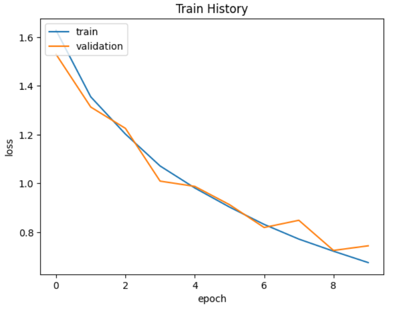
可以发现解决了过拟合的问题
但是准确率并没有提高多少,因为训练周期太少了。
![]()
模型的保存和加载
模型保存
模型训练好了后,使用model.save_weights("文件路径")来保存模型,注意模型后缀为.h5
model.save_weights("E://cifarCnnModel.h5")
print("Save model to disk")
模型加载
使用model.load_weights("文件路径")加载模型
try:
    model.load_weights("E://cifarCnnModel.h5")
    print("加载模型成功!继续训练模型")
except:
    print("加载模型失败!开始训练一个新的模型")
PyTorch版本(飞机和鸟二分类)
安装所需的库
pip install torchvision
pip install matplotlib
导入所需要的库
import torch.nn as nn
import torch
from torchvision import datasets
from torchvision import transforms
import matplotlib.pyplot as plt
import torch.nn.functional as F
import random
import torch.optim as optim
import datetime
导入数据并查看信息
tensor_cifar10 = datasets.CIFAR10(data_path,train=True,download=False,transform=transforms.ToTensor())
img_t,_ = tensor_cifar10[99] #获取索引为99的数据的图片信息和标签信息,标签信息暂时用不到
print( type(img_t) ) #结果显示img_t类型为:<class 'torch.Tensor'>
print( img_t.min() ) #输出img_t中最小的值
print( img_t.max() ) #输出img_t中最大的值
print( img_t.shape ) #输出图片形状,结果为:torch.Size([3, 32, 32])
img_changed=img_t.permute(1,2,0) #改变形状布局,第0维为原本第1维,第1维为原本第2维,第2维为原本第0维,
img_changed.shape # 结果为:torch.Size([32, 32, 3])
plt.imshow(img_changed) #显示图片
plt.show()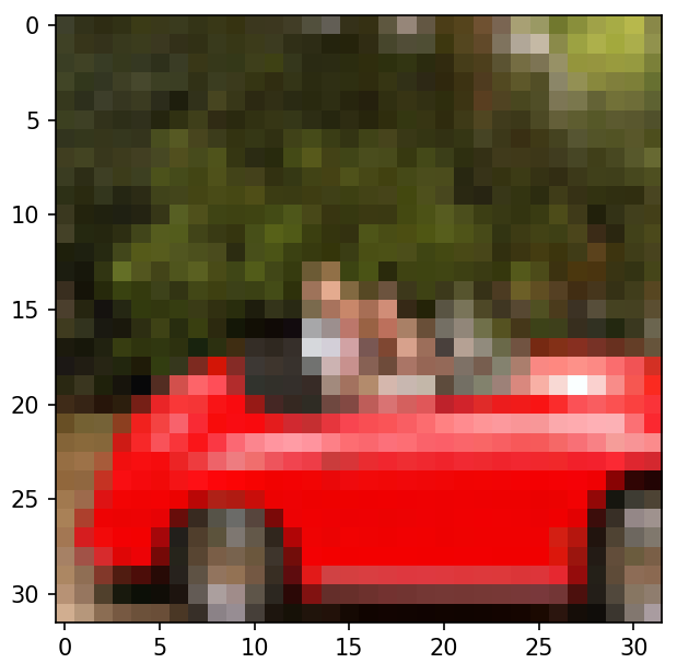
计算每个通道的标准差和平均数
imgs = torch.stack([img_t for img_t,_ in tensor_cifar10],dim=3)#获取所有的图片,放在一个列表中,额外的维度为第3维
print( imgs.shape ) # 结果为:torch.Size([3, 32, 32, 50000]),按照图片通道来摆放
print( imgs.view(3,-1).shape ) #固定第0为3,其他维度合并,结果为:torch.Size([3, 51200000]),将每个通道内合并
print( imgs.view(3,-1).mean(dim=1) ) #计算第1维度的平均数,也就是每个通道的平均数:tensor([0.4914, 0.4822, 0.4465])
print( imgs.view(3,-1).std(dim=1) ) #计算第1维度的方差,每个平均的方差:tensor([0.2470, 0.2435, 0.2616])
torch.Size([3, 32, 32, 50000])
torch.Size([3, 51200000])
tensor([0.4914, 0.4822, 0.4465])
tensor([0.2470, 0.2435, 0.2616])
使用transforms导入数据,对数据进行归一化
transformed_cifar10 = datasets.CIFAR10(data_path,train=True,download=False,transform=transforms.Compose([
transforms.ToTensor(),
transforms.Normalize((0.4914, 0.4822, 0.4465),(0.2470, 0.2435, 0.2616))
#第一组参数为每个通道的平均数,第二组参数为每个通道的方差
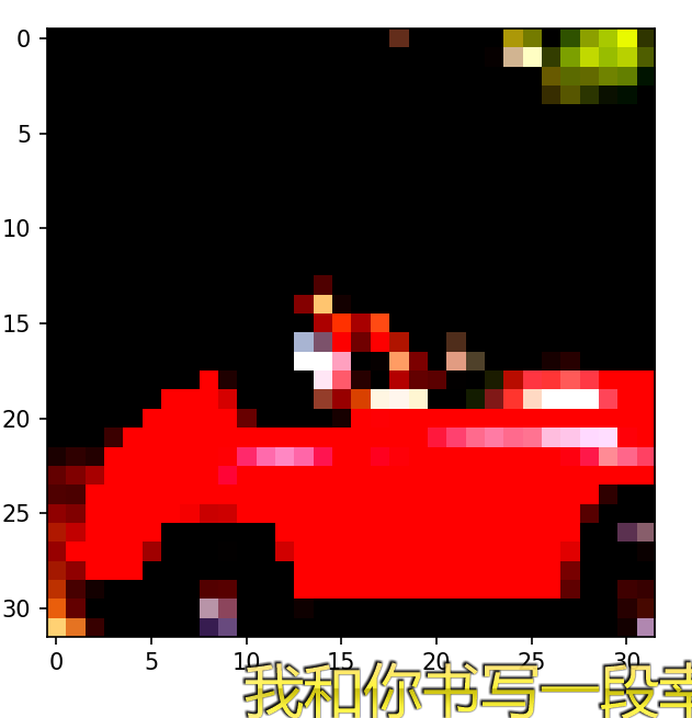
]))查看索引为99的数据的图片
img_t,_ =transformed_cifar10[99] #查看第99张图片
plt.imshow(img_t.permute(1,2,0))
plt.show()
对图片进行归一化后,物体的辨识度更高了
使用归一化方式导入数据
cifar10 = datasets.CIFAR10(data_path,train=True,download=False,transform=transforms.Compose([
    transforms.ToTensor(),
    transforms.Normalize((0.4914, 0.4822, 0.4465),(0.2470, 0.2435, 0.2616))
]))
label_map = {0:0,2:1}  #标签映射,原本鸟和飞机的label为0和2,将其映射为0和1
class_names = ['airplane','bird'] #类别名称
cifar2 = [ (img,label_map[label])
           for img,label in cifar10
           if label in [0,2]
           ] #在cifar10中筛选label为0和2的数据,放在列表中
多层感知机模型
Softmax的定义
Softmax可以将一系列数据压缩到0和1之间,和为1.
x = torch.tensor([1.0,2.0,3.0])
def softmax(x): #手工定义softmax分类函数
    return torch.exp(x)/torch.exp(x).sum()
print(softmax(x).sum()) #输出为tensor(1.)

x = torch.tensor([[1.0,2,3],
                  [1.0,2,3]])
softmax =  nn.Softmax(dim=1) #dim=1,表示对于每个数据的预测进行softmax处理。
print(softmax(x))
#若有多个列表,则将每个列表单独处理。
'''
结果为
tensor([[0.0900, 0.2447, 0.6652],
        [0.0900, 0.2447, 0.6652]])
'''
定义顺序模型
loss = nn.NLLLoss() #损失函数
n_out = 2 #输出类别个数
model = nn.Sequential(
    nn.Linear(3072,512),
    nn.Tanh(),
    nn.Linear(512,n_out),
    nn.Softmax(dim=1)
)
卷积神经网络
导入数据
cifar10 = datasets.CIFAR10(data_path,train=True,download=True,transform=transforms.Compose([
    transforms.ToTensor(),
    transforms.Normalize((0.4914, 0.4822, 0.4465),(0.2470, 0.2435, 0.2616))
]))
label_map = {0:0,2:1}
class_names = ['airplane','bird']
cifar2 = [ (img,label_map[label])
           for img,label in cifar10
           if label in [0,2]
           ]
定义准确率验证函数和批次转换函数
def validate(model,val_data,val_label): #准确率验证函数
    correct =0
    total=0
    device = (torch.device('cuda')) if torch.cuda.is_available() else torch.device('cpu') #能放在GPU运算就放在GPU运算
    with torch.no_grad(): #在不考虑梯度的上下文中计算
        for index in range(len(val_data)-1):
            imgs = val_data[index]
            labels = val_label[index]
            imgs= imgs.to(device=device) #指定CPU或GPU
            labels = labels.to(device=device) #指定CPU或GPU
            output=model(imgs)
            _,predicted=torch.max(output,dim=1) #对第1维求最大数的索引
            total += val_label[index].shape[0] #计算总数据量
            correct+=int( (predicted==labels).sum() ) #计算索引等于标签的数据个数
            #tensor列表之间的等号与list列表之间的等号不同
            #list列表之间用等号返回结果为一个boolean变量,表示列表是否相等
            #tensor列表之间等号返回结果为一个boolean列表,表示每个下标的元素是否相等。例如tensor([ True, False,  True, False,  True])
            #tensor求和时True表示1,Flase表示0
    return correct/total #正确预测所占的比例
def convertToInput(cifarData,batchSize):
    data=[]
    label=[]
    for index in range(0,len(cifarData),batchSize):
        batch_data=[] #每一批次数据
        batch_label=[]#每一批次的标签
        for item in cifarData[index:index+batchSize]: #按批次遍历
            batch_data=batch_data+[item[0]]
            batch_label = batch_label+[item[1]]
        batch_label=torch.tensor(batch_label) #当前批次标签转换为tensor
        label=label+[batch_label] #转换后的tensor放到列表中
        data=data+[ torch.stack(batch_data,dim=0 )] #因为cifar中的img已经是tensor,只需要将每一批次img按照第0维摆放,作为一批放到列表中
    return data,label
定义卷积神经网络
class Net(nn.Module):
    def __init__(self):
        super().__init__()
        self.conv1 = nn.Conv2d(3,16,kernel_size=3,padding=1)
        self.act1 = nn.Tanh()
        self.pool1 = nn.MaxPool2d(2)
        self.conv2 = nn.Conv2d(16,8,kernel_size=3,padding=1)
        self.act2 = nn.Tanh()
        self.pool2 = nn.MaxPool2d(2)
        self.fc1 = nn.Linear(8*8*8,32)
        self.act3 = nn.Tanh()
        self.fc2  = nn.Linear(32,2)
    def forward(self,x):
        out = self.conv1(x)
        out = self.act1(out)
        out = self.pool1(out)
        out = self.conv2(out)
        out = self.act2(out)
        out = self.pool2(out)
        out = out.view(-1,8*8*8)
        out = self.fc1(out)
        out = self.act3(out)
        out = self.fc2(out)
        return out
查看模型参数
torchsummary可以像keras的summary一样查看模型参数
from torchsummary import summary
summary(model,(3,32,32))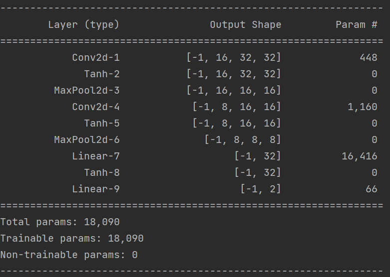
定义训练函数
optimizer = optim.SGD(model.parameters(),lr=1e-2) #优化器为SGD
loss_fn = nn.CrossEntropyLoss() #因为交叉熵损失自带softmax,因此模型最后一层并不需要softmax激活
def training_loop(n_epochs,optimizer,model,loss_fn,cifar2):
    random.shuffle(cifar2) #打乱cifar2数据集
    proportion = int(0.8 * len(cifar2)) #划分训练集和验证集
    cifar2_train = cifar2[:proportion]
    cifar2_val = cifar2[proportion:]
    device = (torch.device('cuda')) if torch.cuda.is_available() else torch.device('cpu') #判断gpu是否可用
    for epoch in range(1,n_epochs+1):
        random.shuffle(cifar2_train) #打乱训练集
        train_data, train_label = convertToInput(cifar2_train, 64) #将训练数据转换为64个为一批
        loss_train=0.0 #训练集损失
        for index in range(len(train_data)-1): #按照批次一批一批的训练,由于最后一批没有64个,因此去除
            imgs=train_data[index] #每一批次的imgs形状为 64 x 3 x 32 x 32
            labels = train_label[index]  #获取每一批次的标签
            imgs=imgs.to(device=device)
            labels=labels.to(device=device)
            outputs = model(imgs)  #模型预测
            loss = loss_fn(outputs,labels) #计算损失
            optimizer.zero_grad()  #清空已有的梯度
            loss.backward() #反向传播计算梯度
            optimizer.step() #跟新模型内部参数parameters
            loss_train += loss.item() #loss为当前批次64个的损失。之后计算损失时要平均到每个样本上
        if epoch == 1 or epoch %10 ==0:
            train_accuracy = validate(model,train_data,train_label) #计算训练集上的准确率
            random.shuffle(cifar2_val) #打乱验证集
            val_data, val_label=convertToInput(cifar2_val,64)
            val_accuracy = validate(model, val_data, val_label) #计算验证集上的准确率
            print('{}:Epoch:{}, Training loss:{:.4f}, Train_Accuracy:{:.4f},Validation_Accuracy:{:.4f}'.format(
                datetime.datetime.now(), #输出当前时间
                epoch, #输出周期数
                loss_train/(len(train_data)-1)*64,  #输出每个样本的平均损失
                train_accuracy, #输出训练集准确率
                val_accuracy #输出验证集准确率
            ))
训练模型
training_loop(
    n_epochs=100,
    optimizer= optimizer,
    model=model,
    loss_fn=loss_fn,
    cifar2=cifar2
)
使用带有BatchNormalization和Dropout的模型
class Net(nn.Module):
    def __init__(self,n_chanels=32):
        super().__init__()
        self.n_chanels=n_chanels
        self.conv1 = nn.Conv2d(3,n_chanels,kernel_size=3,padding=1,bias=False) #BatchNorm会消除bias的影响,因此后面带有BN层,前面不需要偏置项
        self.conv1_batchnorm = nn.BatchNorm2d(num_features=n_chanels)
        self.conv1_dropout = nn.Dropout2d(p=0.4)
        self.conv2 = nn.Conv2d(n_chanels,n_chanels//2,kernel_size=3,padding=1,bias=False)
        self.conv2_batchnorm = nn.BatchNorm2d(num_features=n_chanels//2)
        self.conv2_dropout = nn.Dropout(p=0.4)
        self.fc1 = nn.Linear(8*8*n_chanels//2,32)
        self.fc2  = nn.Linear(32,2)

    def forward(self,x):
        out = self.conv1(x)
        out = self.conv1_batchnorm(out)
        out = torch.tanh(out)
        out = F.max_pool2d(out,2)
        out = self.conv1_dropout(out)

        out = self.conv2(out)
        out = self.conv2_batchnorm(out)
        out = torch.tanh(out)
        out = F.max_pool2d(out, 2)
        out = self.conv2_dropout(out)

        out = out.view(-1,8*8*self.n_chanels//2)
        out = self.fc1(out)
        out = torch.tanh(out)
        out = self.fc2(out)
        return out
残差神经网络
class ResBlock(nn.Module):
    def __init__(self,n_chans):
        super(ResBlock, self).__init__()
        self.conv = nn.Conv2d(n_chans,n_chans,kernel_size=3,padding=1,bias=False)
        #BN层会消除bias的影响,因此通常前一层不需要偏差,减少计算。
        self.batch_norm = nn.BatchNorm2d(num_features=n_chans)
        nn.init.kaiming_normal_(self.conv.weight,nonlinearity='relu')
        #正态随机元素初始化
        nn.init.constant_(self.batch_norm.weight,0.5)
        #bach生成0平均数,0.5方差的输出
        nn.init.zeros_(self.batch_norm.bias)
    def forward(self,x):
        out = self.conv(x)
        out = self.batch_norm(out)
        out = torch.relu(out)
        return out + x

class NetResDeep(nn.Module):
    def __init__(self,n_chansl=32,n_blocks=10):#n_blocks表示残差块的个数
        super().__init__()
        self.n_chans = n_chansl
        self.conv1 = nn.Conv2d(3,n_chansl,kernel_size=3,padding=1)
        self.resblocks = nn.Sequential(
            *(n_blocks * [ResBlock(n_chansl=n_chansl)])) #n_blocks*()表示[]中复制10份,最终得到一个列表[...],再用*号提取参数,一个个传入函数
        self.fc1 = nn.Linear(8*8*n_chansl,32)
        self.fc2 = nn.Linear(32,2)

    def forward(self,x):
        out = self.conv1(x)
        out = torch.relu(out)
        out = F.max_pool2d(out,2)
        out = self.resblocks(out)
        out = F.max_pool2d(out,2)
        out = out.view(-1,8*8*self.n_chans)
        out = self.fc1(out)
        out = torch.relu(out)
        out = self.fc2(out)
        return out
模型形状
----------------------------------------------------------------
Layer (type) Output Shape Param #
================================================================
Conv2d-1 [-1, 32, 32, 32] 896
Conv2d-2 [-1, 32, 16, 16] 9,216
BatchNorm2d-3 [-1, 32, 16, 16] 64
ResBlock-4 [-1, 32, 16, 16] 0
Conv2d-5 [-1, 32, 16, 16] 9,216
BatchNorm2d-6 [-1, 32, 16, 16] 64
ResBlock-7 [-1, 32, 16, 16] 0
Conv2d-8 [-1, 32, 16, 16] 9,216
BatchNorm2d-9 [-1, 32, 16, 16] 64
ResBlock-10 [-1, 32, 16, 16] 0
Conv2d-11 [-1, 32, 16, 16] 9,216
BatchNorm2d-12 [-1, 32, 16, 16] 64
ResBlock-13 [-1, 32, 16, 16] 0
Conv2d-14 [-1, 32, 16, 16] 9,216
BatchNorm2d-15 [-1, 32, 16, 16] 64
ResBlock-16 [-1, 32, 16, 16] 0
Conv2d-17 [-1, 32, 16, 16] 9,216
BatchNorm2d-18 [-1, 32, 16, 16] 64
ResBlock-19 [-1, 32, 16, 16] 0
Conv2d-20 [-1, 32, 16, 16] 9,216
BatchNorm2d-21 [-1, 32, 16, 16] 64
ResBlock-22 [-1, 32, 16, 16] 0
Conv2d-23 [-1, 32, 16, 16] 9,216
BatchNorm2d-24 [-1, 32, 16, 16] 64
ResBlock-25 [-1, 32, 16, 16] 0
Conv2d-26 [-1, 32, 16, 16] 9,216
BatchNorm2d-27 [-1, 32, 16, 16] 64
ResBlock-28 [-1, 32, 16, 16] 0
Conv2d-29 [-1, 32, 16, 16] 9,216
BatchNorm2d-30 [-1, 32, 16, 16] 64
ResBlock-31 [-1, 32, 16, 16] 0
Linear-32 [-1, 32] 65,568
Linear-33 [-1, 2] 66
================================================================
Total params: 159,330
Trainable params: 159,330
Non-trainable params: 0
----------------------------------------------------------------
Input size (MB): 0.01
Forward/backward pass size (MB): 2.13
Params size (MB): 0.61
Estimated Total Size (MB): 2.74
----------------------------------------------------------------
本文来自博客园,作者:Laplace蒜子,转载请注明原文链接:https://www.cnblogs.com/RedNoseBo/p/17192410.html

 浙公网安备 33010602011771号