Lending Club 贷款业务信用评分卡建模

目前，国内外对个人信用风险评估模型的研究方法，是通过用户的历史行为（如历史数据的多维特征和贷款状态是否违约）来训练模型，通过这个模型对新增的贷款人“是否具有偿还能力，是否具有偿债意愿”进行分析，预测贷款申请人是否会发生违约贷款。主要有两种方法：以 Logistic 回归模型为代表的传统信用风险评估方法；以支持向量机、神经网络、决策树等机器学习理论为代表的新型信用风险评估模型。

本文『以Logistic 回归模型建立信用评分卡模型』方法对 Lending Club 公司贷款业务进行信用卡评分建模，通过模型预测贷款人是否会违约，达到最小化风险的目的。其原理是将模型变量 WOE 编码方式离散化之后运用 logistic 回归模型进行的一种二分类变量的广义线性模型。一般地，我们将模型目标标量 1 记为违约用户，目标变量 0 记为正常用户。

原始数据来源：https://www.kaggle.com/wendykan/lending-club-loan-data/kernels
原始时间跨度：2007-2015
原始数据维度：226万 * 145
本项违约定义：违约16天及其以上（d_loan = [ "Late (16-30 days)" , "Late (31-120 days)"，"Charged Off" , "Default", "Does not meet the credit policy. Status:Charged Off"]）
模型时间窗口：由于数据量较大，时间跨度过长，故选择2016、2017 两年的数据进行后续建模（数据877986*145）。

对 Lending Club 公司业务前期分析：

Lending Club 公司2007-2018贷款业务初步分析：https://www.cnblogs.com/Ray-0808/p/12618551.html
Lending Club 公司2007-2018贷款业务好坏帐分析：https://www.cnblogs.com/Ray-0808/p/12668594.html

1. 数据清洗

1.1 删除变量

删去缺失率大于 25% 变量（44个变量）
删去取值只有一个的变量,同一性很大的变量（17个变量）
删去一些无用变量，例如一些贷后数据，如下图

1.2 删除记录缺失

25% 特征信息的记录（1条记录）
剔除包含异常值的记录

1.3 填充空值

缺失值标示为一类，将字符型缺失数据填充 'UnKnown'
众数填充，将数值型缺失数据用众数填充

清洗后数据量：数据877985*71

2. 数据分箱

2.1 数据分箱方法

数据分箱的方法可以分为：有监督分箱和无监督分箱。有监督分箱可以分为 Split 分箱和 Merge 分箱，无监督分箱为等频分箱、等距分箱、聚类分箱等。
本项目使用卡方分箱法（ChiMerge），基本思想是如果两个相邻的区间具有类似的类分布，则这两个区间合并；否则，它们应保持分开。
操作过程：

输入：分箱的最大区间数n
初始化
- 连续值按升序排列，离散值先转化为坏客户的比率，然后再按升序排列；
- 为了减少计算量，对于状态数大于某一阈值 (建议为100) 的变量，利用等频分箱进行粗分箱。
- 若有缺失值，则缺失值单独作为一个分箱。
合并区间
- 计算每一对相邻区间的卡方值；
- 将卡方值最小的一对区间合并
- 重复以上两个步骤，直到分箱数量不大于n
分箱后处理
- 对于坏客户比例为 0 或 1 的分箱进行合并 (一个分箱内不能全为好客户或者全为坏客户)。
- 对于分箱后某一箱样本占比超过 95% 的箱子进行删除。
输出：分箱后的数据和分箱区间。

2.2 本项目数据划分

由于使用的卡方分箱法，分箱过程中会使用到实际违约变量（"y_label"）的数据，为防止数据泄露，需要在对数据进行分箱前划分数据集。这里由于数据倾斜（违约样本占比远少于正常样本），所以使用分层抽样的方法，避免数据分布不均。

1 # 分层抽样, 避免不均
2 from sklearn.model_selection import StratifiedShuffleSplit
3 split = StratifiedShuffleSplit(n_splits=1, test_size=0.2, random_state=42)
4 for train_index, test_index in split.split(data, data.loc[:, 'y_label']):
5     train_set = data.iloc[train_index, :]
6     test_set = data.iloc[test_index, :]

View Code

2.3 本项目分箱流程

类别型变量
1. 当取值较少时：
  1. 如果每种类别同时包含好坏样本，无需分箱
  2. 如果有类别只包含好坏样本的一种，需要合并
2. 当取值较多时，先用bad rate编码（即将每个类别变量的不同值用其违约率代替），再用连续型分箱的方式进行分箱
连续型变量
1. 检查是否有特殊值，需要单独分箱
2. 检查原始分箱个数，如果过大，需要粗分箱（比如100箱）
3. 使用卡方分箱法
4. 检查所分箱是否有箱是相同值，有则合并
5. 检查分箱后是否符合单调性，不单调则合并

本部代码较多，集中放置于附录代码中。

3. WOE 编码

在分箱完毕后，需要对每个变量的各箱进行编码，才能送入逻辑回归模型中进行使用。
WOE的全称是“Weight of Evidence”,计算每个变量的每箱 WOE 值，然后使用对应 WOE 值对该变量进行编码。其不同于ONE-HOT编码后会创建许多新变量，造成矩阵稀疏、维度灾难等问题
WOE 编码相当于把分箱后的特征从非线性可分映射到近似线性可分的空间内：

可提升模型的预测效果
将自变量规范到同一尺度上
WOE能反映自变量取值的贡献情况
有利于对变量的每个分箱进行评分
转化为连续变量之后，便于分析变量与变量之间的相关性
与独热向量编码相比，可以保证变量的完整性，同时避免稀疏矩阵和维度灾难

如 ”int_rate“ 变量：

4. 变量筛选

4.1 单变量筛选

基于 IV 值的变量筛选信息价值，类似于信息增益、基尼系数
基于 stepwise 的变量筛选，一步一步进行变量筛选
基于特征重要度的变量筛选：RF, GBDT…
基于 LASSO 正则化的变量筛选

本文对比使用了两种，最终选择第一种方法。

 1 # 4.1 单变量选择  -->  按 IV 值挑选变量，IV > 0.02
 2 high_IV = {k: v for k, v in IV_dict.items() if v >= 0.02}
 3 high_IV_dict_sorted = sorted(high_IV.items(), key=lambda x: x[1], reverse=False)
 4 high_IV_values = [i[1] for i in high_IV_dict_sorted]
 5 high_IV_names = [i[0] for i in high_IV_dict_sorted]
 6 feat_select_1 = []
 7 for i in high_IV_names:
 8     feat_select_1.append(i + '_WOE')
 9 print("经过 IV>0.02 挑选后，有 {} 个变量".format(len(feat_select_1)))
10 print("这些变量是：", feat_select_1)
11 fig_1, ax = plt.subplots(1, 1)
12 plt.barh(range(len(high_IV_values)), high_IV_values)
13 plt.title('feature IV')
14 plt.yticks(range(len(high_IV_names)), high_IV_names)
15 plt.savefig(folder_data + "feature_IV.png", dpi=1000, bbox_inches='tight')  # 解决图片不清晰，不完整的问题
16 # plt.show()

查看基于IV值挑选变量的代码

 1 # 4.2 单变量选择  -->  随机森林法选择变量
 2 X = train_data[WOE_feat]
 3 X = np.matrix(X)
 4 y = train_data['y_label']
 5 y = np.array(y)
 6 RFC = RandomForestClassifier()
 7 RFC_Model = RFC.fit(X, y)
 8 features_rfc = train_data[WOE_feat].columns
 9 RF_feat_importance = {features_rfc[i]: RFC_Model.feature_importances_[i] for i in range(len(features_rfc))}
10 RF_feat_importance_sorted = sorted(RF_feat_importance.items(), key=lambda x: x[1], reverse=False)
11 RF_feat_values = [i[1] for i in RF_feat_importance_sorted]
12 RF_feat_names = [i[0] for i in RF_feat_importance_sorted]
13 print("经过随机森林法单变量挑选后，有 {} 个变量".format(len(RF_feat_names)))
14 print("这些变量是：", RF_feat_names)
15 fig_2, ax = plt.subplots(1, 1)
16 plt.barh(range(len(RF_feat_values)), RF_feat_values)
17 plt.title('随机森林特征重要性排行')
18 plt.yticks(range(len(RF_feat_names)), RF_feat_names)
19 plt.show()

查看基于随机森林法挑选变量的代码

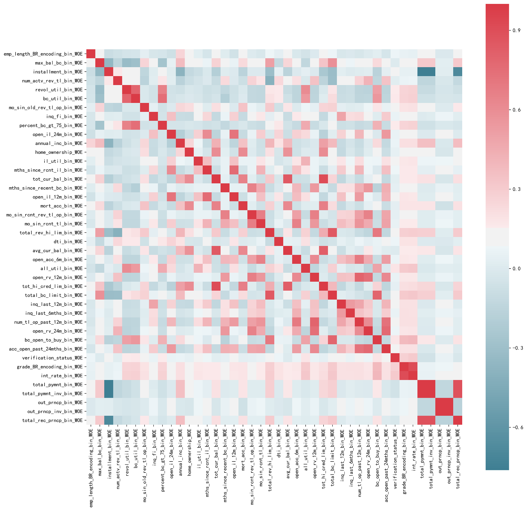
4.2 变量相关性

双变量相关性线性相关性：皮尔逊相关系数
多变量相关性多重共线性：某一个变量可以由其他变量线性表示，使用VIF（方差膨胀因子）检验

下图变量线性相关性热力图：

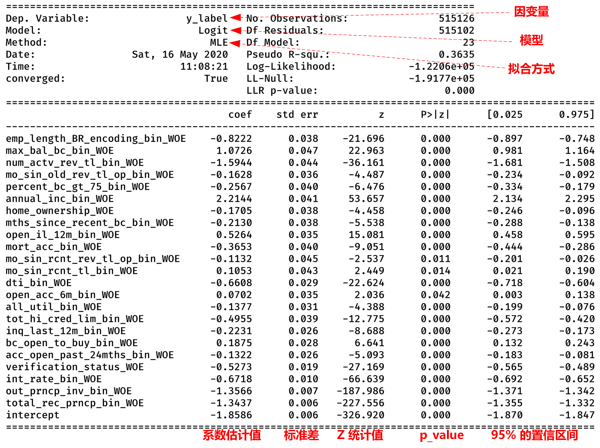
5. 建模评价

5.1 建模

可以使用 sklearn 或者 statsmodels 等等库调用逻辑回归模型。

5.2 评价

		预测
		1	0
实际	1	TP（true positivie）	FN（false negative）
实际	0	FP（false positive）	TN（true negative）

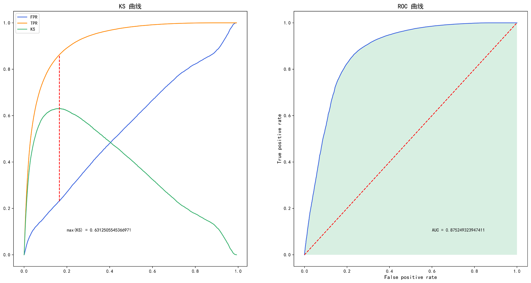
真正率（TPR）：实际上为正例被预测为正例的比率，TPR = TP / (TP + FN)
假正率（FPR）：实际上为反例被预测为正例的比率，FPR = FP / (FP + TN)
ROC 曲线：横坐标由假正率，纵坐标由真正率构成的曲线
AUC 值：ROC 曲线到坐标轴之间的面积，指随机给定一个正样本和一个负样本，分类器输出该正样本为正的那个概率值比分类器输出该负样本为正的那个概率值要大的可能性
KS 值：KS = max(TPR-FPR)，大于0.2 则说明模型区分性较好

6. 参考文献

逻辑回归算法：https://www.cnblogs.com/biyeymyhjob/archive/2012/07/18/2595410.html
特征重要度 WoE、IV、BadRate：https://www.cnblogs.com/Allen-rg/p/11507970.html
随机森林： https://www.cnblogs.com/maybe2030/p/4585705.html#top
L1、L2：https://blog.csdn.net/jinping_shi/article/details/52433975
玩转逻辑回归之金融评分卡模型：https://zhuanlan.zhihu.com/p/36539125
利用LendingClub数据建模：https://zhuanlan.zhihu.com/p/21550547

附录：

  1 # coding:utf-8
  2 
  3 import pandas as pd
  4 import numpy as np
  5 import time
  6 import matplotlib.pyplot as plt
  7 import seaborn as sns
  8 from statsmodels.stats.outliers_influence import variance_inflation_factor
  9 import pickle
 10 from sklearn.model_selection import train_test_split
 11 import statsmodels.api as sm
 12 from sklearn.ensemble import RandomForestClassifier
 13 import CustomFunction as cf
 14 from sklearn.model_selection import StratifiedShuffleSplit
 15 
 16 # 显示设置
 17 plt.rcParams['font.sans-serif'] = ['SimHei']  # 用来正常显示中文标签
 18 plt.rcParams['axes.unicode_minus'] = False  # 用来正常显示负号,#有中文出现的情况，需要u'内容'
 19 pd.set_option('display.max_columns', 1000)
 20 pd.set_option('display.width', 1000)
 21 pd.set_option('display.max_colwidth', 1000)
 22 pd.set_option('display.max_row', 1000)
 23 
 24 # 程序开始时间计算
 25 start_time = time.process_time()
 26 
 27 # 存放数据文件路径
 28 folder_data = r'E:/3.Python_Project/LENGING_CLUB/data/'
 29 
 30 # ----------------------------------------------------------------------------------------------------------------------
 31 # 0. 读取数据 ， 转换数据格式
 32 # ----------------------------------------------------------------------------------------------------------------------
 33 # loan = pd.read_csv('loan.csv', low_memory=False)
 34 # df = loan.copy()
 35 #
 36 # # 将 ‘issue_d’ str形式的时间日期转换
 37 # dt_series = pd.to_datetime(df['issue_d'])
 38 # df['year'] = dt_series.dt.year
 39 # df['month'] = dt_series.dt.month
 40 #
 41 # # 取 2016-2017 年度的数据进行后续计算
 42 # print(df['year'].unique())
 43 # df = df[df['year'].isin([2016, 2017])]
 44 # print(df['year'].unique())
 45 #
 46 # # 根据贷款状态 ‘loan_status’ 定义违约标签
 47 # d_loan = ["Late (16-30 days)", "Late (31-120 days)", "Charged Off", "Default",
 48 #           "Does not meet the credit policy. Status:Charged Off"]
 49 # df['loan_condition'] = np.nan
 50 # lst = [df]
 51 #
 52 #
 53 # def loan_condition(status):
 54 #     if status in d_loan:
 55 #         return 'd Loan'
 56 #     else:
 57 #         return 'c Loan'
 58 #
 59 #
 60 # df['loan_condition'] = df['loan_status'].apply(loan_condition)
 61 # df['y_label'] = np.nan
 62 # for col in lst:
 63 #     col.loc[df['loan_condition'] == 'c Loan', 'y_label'] = 0  # 正常贷款
 64 #     col.loc[df['loan_condition'] == 'd Loan', 'y_label'] = 1  # 违约贷款
 65 # df['y_label'] = df['y_label'].astype(int)
 66 # df.to_pickle(folder_data + "loan_1617_preprocessing.pkl")
 67 
 68 # ----------------------------------------------------------------------------------------------------------------------
 69 # 1. 数据清洗
 70 # ----------------------------------------------------------------------------------------------------------------------
 71 # df = pd.read_pickle(folder_data+"loan_1617_preprocessing.pkl")
 72 #
 73 # # 1.1 删除变量
 74 # df_na = df.isna().sum()/df.shape[0]     # 缺失率
 75 # # 删去缺失率大于 25% 变量
 76 # del_var = []
 77 # var_big_na = list(df_na[df_na>0.25].index ) # 缺失值超过 25% 的变量
 78 # del_var.append(var_big_na)
 79 # df.drop(var_big_na,axis=1,inplace=True)
 80 # df_na.drop(var_big_na,axis=0,inplace=True)
 81 # # 删去特征只有一个的变量,同一性很大的变量
 82 # var_same=[]
 83 # for i in df.columns:
 84 #     mode_value = df[i].mode()[0]
 85 #     mode_rate = len(df[i][df[i]==mode_value]) / df.shape[0]
 86 #     if mode_rate > 0.9:
 87 #         var_same.append(i)
 88 #         df.drop(i,axis=1,inplace=True)
 89 # del_var.append(var_same)
 90 # # 删去自选的一些无用特特征
 91 # var_no_use = ['sub_grade', 'emp_title', 'addr_state', 'zip_code', 'loan_condition', 'loan_status',
 92 #               'last_pymnt_d', 'last_credit_pull_d', 'last_pymnt_amnt', 'earliest_cr_line',
 93 #               'initial_list_status', 'title', 'issue_d', 'mths_since_recent_inq']
 94 # del_var.append(var_no_use)
 95 # df.drop(var_no_use,axis=1,inplace=True)
 96 #
 97 # # 1.2 删除记录
 98 # df_na_row = df.isna().sum(axis=1)/df.shape[1]
 99 # del_row = list(df_na_row[df_na_row>0.25].index ) # 信息缺失超过 25% 的记录
100 # df.drop(del_row,axis=0,inplace=True)
101 #
102 # # 1.3 缺失值填充
103 # # 查看变量类型是否正确,并填充缺失值
104 # object_columns = df.select_dtypes(include=["object"]).columns
105 # numeric_columns = df.select_dtypes(exclude=["object"]).columns
106 # # print(df[object_columns].head())
107 # # print(df[numeric_columns].head())
108 #
109 # # 将字符型缺失数据填充 'UnKnown'
110 # df[object_columns]=df[object_columns].fillna('UnKnown')
111 #
112 # # 将数值型缺失数据用众数填充
113 # for i in numeric_columns:
114 #     mode_value = df[i].mode()[0]
115 #     df[i] = df[i].fillna(mode_value)
116 #
117 # print("数据清洗后有{}个变量".format(df.shape[1]-3))
118 # print("数据清洗后有{}条记录".format(df.shape[0]))
119 # df.to_pickle(folder_data+"loan_1617_clean.pkl")
120 
121 # ----------------------------------------------------------------------------------------------------------------------
122 # 2. 数据分箱(ChiMerge)
123 # ----------------------------------------------------------------------------------------------------------------------
124 # 分箱之后：
125 # （1）不超过5箱
126 # （2）Bad Rate单调
127 # （3）每箱同时包含好坏样本
128 # （4）特殊值如'UnKnown'单独成一箱
129 # ----------------------------------------------------------------------------------------------------------------------
130 loan_clean = pd.read_pickle(folder_data + "loan_1617_clean.pkl")
131 # print(loan_clean.head())
132 # print(loan_clean.isnull().sum())
133 loan_clean = loan_clean[loan_clean['dti'] != -1]
134 data = loan_clean.loc[loan_clean['term'] == ' 36 months'].copy()
135 data.drop(['year', 'month', 'term'], axis=1, inplace=True)
136 
137 num_features = list(data.select_dtypes(exclude=["object"]).columns)  # 数值变量
138 cat_features = list(data.select_dtypes(include=["object"]).columns)  # 类型变量
139 # print(num_features)
140 # print(cat_features)
141 #
142 # 划分数据集
143 # train_data, test_data = train_test_split(data, test_size=0.4)
144 # 分层抽样, 避免不均
145 split = StratifiedShuffleSplit(n_splits=1, test_size=0.2, random_state=42)
146 for train_index, test_index in split.split(data, data.loc[:, 'y_label']):
147     train_set = data.iloc[train_index, :]
148     test_set = data.iloc[test_index, :]
149 
150 # 有几个字段的值比较少,剔除掉
151 train_set = train_set[~(train_set['home_ownership'] == 'NONE')]
152 train_set = train_set[~(train_set['purpose'].isin(['wedding', 'educational']))]
153 train_data = train_set.copy()
154 test_set = test_set[~(test_set['home_ownership'].isin(['NONE']))]
155 test_set = test_set[~(test_set['purpose'].isin(['wedding', 'educational']))]
156 test_data = test_set.copy()
157 
158 # 2.1 处理类型变量
159 cat_more_5_feat = []  # 类型变量中超过 5 种取值的变量
160 cat_less_5_feat = []  # 类型变量中超过 5 种取值的变量
161 # a) 检查类型变量中哪些变量取值超过5
162 for var in cat_features:
163     value_counts = data[var].nunique()
164     if value_counts > 5:
165         cat_more_5_feat.append(var)
166     else:
167         cat_less_5_feat.append(var)
168 
169 # b) 对于类型变量值分类小于5的变量，其每种类别应该包含好坏两种样本，如果只有其中一种样本则需要合并
170 merge_bin_dict = {}  # 存放需要合并的变量，以及合并方法
171 for var in cat_less_5_feat:
172     bin_bad_rate = cf.BinBadRate(train_data, var, 'y_label')[0]
173     if min(bin_bad_rate.values()) == 0:
174         print('{} 类型变量需要合并箱'.format(var))
175         combine_bin = cf.MergeBin(train_data, var, 'y_label')
176         merge_bin_dict[var] = combine_bin
177         pass
178     if max(bin_bad_rate.values()) == 1:
179         print('{} 类型变量需要合并箱'.format(var))
180         combine_bin = cf.MergeBin(train_data, var, 'y_label', direction='good')
181         merge_bin_dict[var] = combine_bin
182 #
183 # print(merge_bin_dict)
184 #
185 # # c） 对于类型变量值分类大于5的变量，使用 badrate 编码，放入连续型变量
186 # for var in cat_more_5_feat:
187 #     if 'UnKnown' in list(data[var].unique()):
188 #         encoding_df = train_data.loc[train_data[var] != 'UnKnown'].copy()
189 #     else:
190 #         encoding_df = train_data.copy()
191 #     bin_bad_rate = cf.BinBadRate(encoding_df, var, 'y_label')[0]
192 #     if 'UnKnown' in list(data[var].unique()):
193 #         bin_bad_rate['UnKnown'] = -1
194 #     new_var = var + '_BR_encoding'
195 #     num_features.append(new_var)
196 #     train_data[new_var] = train_data[var].map(lambda x: bin_bad_rate[x])
197 #     test_data[new_var] = test_data[var].map(lambda x: bin_bad_rate[x])
198 #
199 # # 2.2 对连续变量进行卡方分箱（chimerge）
200 # bin_feat = []
201 # for var in num_features:
202 #     print("请稍等，正在处理 {} 字段".format(var))
203 #     if -1 not in train_data[var].unique():
204 #         max_bin_num = 5  # 设置最大分箱数
205 #         split_points = cf.ChiMerge(train_data, var, 'y_label', max_bin_num=max_bin_num)
206 #         train_data[var + '_bin'] = train_data[var].map(lambda x: cf.AssignBin(x, split_points))
207 #         monotone = cf.BadRateMonotone(train_data, var + '_bin', 'y_label')
208 #         while not monotone:
209 #             max_bin_num -= 1
210 #             split_points = cf.ChiMerge(train_data, var, 'y_label', max_bin_num=max_bin_num)
211 #             train_data[var + '_bin'] = train_data[var].map(lambda x: cf.AssignBin(x, split_points))
212 #             monotone = cf.BadRateMonotone(train_data, var + '_bin', 'y_label')
213 #             # if max_bin_num == 2:
214 #             #     # 当分箱数为2时，必然单调,退出
215 #             #     break
216 #         new_var = var + '_bin'
217 #         bin_feat.append(new_var)
218 #         test_data[var + '_bin'] = test_data[var].map(lambda x: cf.AssignBin(x, split_points))
219 #     else:
220 #         max_bin_num = 5  # 设置最大分箱数
221 #         split_points = cf.ChiMerge(train_data, var, 'y_label', special_attribute=[-1], max_bin_num=max_bin_num)
222 #         train_data[var + '_bin'] = train_data[var].map(lambda x: cf.AssignBin(x, split_points, special_attribute=[-1]))
223 #         monotone = cf.BadRateMonotone(train_data, var + '_bin', 'y_label', special_attribute=[-1])
224 #         while not monotone:
225 #             max_bin_num -= 1
226 #             split_points = cf.ChiMerge(train_data, var, 'y_label', special_attribute=[-1], max_bin_num=max_bin_num)
227 #             train_data[var + '_bin'] = train_data[var].map(lambda x: cf.AssignBin(x, split_points,
228 #                                                                                   special_attribute=[-1]))
229 #             monotone = cf.BadRateMonotone(train_data, var + '_bin', 'y_label', special_attribute=[-1])
230 #         new_var = var + '_bin'
231 #         bin_feat.append(new_var)
232 #         test_data[var + '_bin'] = test_data[var].map(lambda x: cf.AssignBin(x, split_points, special_attribute=[-1]))
233 #
234 # train_data.to_pickle(folder_data + 'train_data_1617.pkl')
235 # test_data.to_pickle(folder_data + 'test_data_1617.pkl')
236 #
237 # bin_feat.sort()
238 # print(bin_feat)
239 # print(train_data.head())
240 
241 # ----------------------------------------------------------------------------------------------------------------------
242 # 3. WOE 编码，计算 IV
243 # ----------------------------------------------------------------------------------------------------------------------
244 train_data = pd.read_pickle(folder_data + 'train_data_1617.pkl')
245 test_data = pd.read_pickle(folder_data + 'test_data_1617.pkl')
246 
247 # print(train_data.head())
248 # print(test_data.head())
249 
250 num_features.remove('y_label')
251 for var in cat_more_5_feat:
252     new_var = var + '_BR_encoding'
253     num_features.append(new_var)
254 bin_feat = []  # bin_feat 分箱后变量
255 for var in num_features:
256     var_bin = var + '_bin'
257     bin_feat.append(var_bin)
258 bin_feat = bin_feat + cat_less_5_feat  # 少于5个不同值的类型变量在本例中不用合并箱，直接使用原分箱即可
259 bin_feat.sort()
260 
261 print("经过分箱后，有 {} 个变量".format(len(bin_feat)))
262 print("这些变量是：", bin_feat)
263 
264 # 计算每个变量分箱后的 WOE 和 IV 值
265 WOE_dict = {}
266 IV_dict = {}
267 for var in bin_feat:
268     WOE_IV = cf.CalcWOE(train_data, var, 'y_label')
269     WOE_dict[var] = WOE_IV['WOE']
270     IV_dict[var] = WOE_IV['IV']
271 
272 # WOE 编码
273 WOE_feat = []
274 for var in IV_dict.keys():
275     var_WOE = var + '_WOE'
276     train_data[var_WOE] = train_data[var].map(WOE_dict[var])
277     test_data[var_WOE] = test_data[var].map(WOE_dict[var])
278     WOE_feat.append(var_WOE)
279 
280 # print(train_data[WOE_feat].head())
281 
282 # ----------------------------------------------------------------------------------------------------------------------
283 # 4. 变量选择
284 # ----------------------------------------------------------------------------------------------------------------------
285 # 4.1 单变量选择  -->  按 IV 值挑选变量，IV > 0.02
286 high_IV = {k: v for k, v in IV_dict.items() if v >= 0.02}
287 high_IV_dict_sorted = sorted(high_IV.items(), key=lambda x: x[1], reverse=False)
288 high_IV_values = [i[1] for i in high_IV_dict_sorted]
289 high_IV_names = [i[0] for i in high_IV_dict_sorted]
290 
291 feat_select_1 = []
292 for i in high_IV_names:
293     feat_select_1.append(i + '_WOE')
294 print("经过 IV>0.02 挑选后，有 {} 个变量".format(len(feat_select_1)))
295 print("这些变量是：", feat_select_1)
296 
297 fig_1, ax = plt.subplots(1, 1, figsize=(10, 10))
298 plt.barh(range(len(high_IV_values[0:19])), high_IV_values[0:19], facecolor='royalblue')
299 plt.title('feature IV')
300 plt.yticks(range(len(high_IV_names[0:19])), high_IV_names[0:19])
301 plt.savefig(folder_data + "feature_IV.png", dpi=1000, bbox_inches='tight')  # 解决图片不清晰，不完整的问题
302 # plt.show()
303 
304 # 4.2 单变量选择  -->  随机森林法选择变量
305 # X = train_data[WOE_feat]
306 # X = np.matrix(X)
307 # y = train_data['y_label']
308 # y = np.array(y)
309 #
310 # RFC = RandomForestClassifier()
311 # RFC_Model = RFC.fit(X, y)
312 #
313 # features_rfc = train_data[WOE_feat].columns
314 # RF_feat_importance = {features_rfc[i]: RFC_Model.feature_importances_[i] for i in range(len(features_rfc))}
315 # RF_feat_importance_sorted = sorted(RF_feat_importance.items(), key=lambda x: x[1], reverse=False)
316 # RF_feat_values = [i[1] for i in RF_feat_importance_sorted]
317 # RF_feat_names = [i[0] for i in RF_feat_importance_sorted]
318 #
319 # print("经过随机森林法单变量挑选后，有 {} 个变量".format(len(RF_feat_names)))
320 # print("这些变量是：", RF_feat_names)
321 #
322 # fig_2, ax = plt.subplots(1, 1)
323 # plt.barh(range(len(RF_feat_values)), RF_feat_values)
324 # plt.title('随机森林特征重要性排行')
325 # plt.yticks(range(len(RF_feat_names)), RF_feat_names)
326 # plt.show()
327 
328 # 4.3 两两变量之间的线性相关性检测
329 # 计算相关系数矩阵，并画出热力图进行数据可视化
330 train_data_WOE = train_data[feat_select_1]
331 corr = train_data_WOE.corr()
332 # print(corr)
333 
334 fig, ax = plt.subplots(figsize=(16, 16))
335 sns.heatmap(corr, mask=np.zeros_like(corr, dtype=np.bool), cmap=sns.diverging_palette(220, 10, as_cmap=True),
336             square=True, ax=ax)
337 plt.savefig(folder_data + "相关性热力图.png", dpi=1000, bbox_inches='tight')  # 解决图片不清晰，不完整的问题
338 # plt.show()
339 
340 # 1，将候选变量按照IV进行降序排列
341 # 2，计算第i和第i+1的变量的线性相关系数
342 # 3，对于系数超过阈值的两个变量，剔除IV较低的一个
343 deleted_index = []
344 cnt_vars = len(high_IV_dict_sorted)
345 for i in range(cnt_vars):
346     if i in deleted_index:
347         continue
348     x1 = high_IV_dict_sorted[i][0] + "_WOE"
349     for j in range(cnt_vars):
350         if i == j or j in deleted_index:
351             continue
352         y1 = high_IV_dict_sorted[j][0] + "_WOE"
353         roh = corr.loc[x1, y1]
354         if abs(roh) > 0.7:
355             x1_IV = high_IV_dict_sorted[i][1]
356             y1_IV = high_IV_dict_sorted[j][1]
357             if x1_IV > y1_IV:
358                 deleted_index.append(j)
359             else:
360                 deleted_index.append(i)
361 
362 feat_select_2 = [high_IV_dict_sorted[i][0] + "_WOE" for i in range(cnt_vars) if i not in deleted_index]
363 
364 print("经过两两共线性挑选后，有 {} 个变量".format(len(feat_select_2)))
365 print("这些变量是：", feat_select_2)
366 
367 # 4.4 多重共线性分析
368 x = np.matrix(train_data[feat_select_2])
369 VIF_list = [variance_inflation_factor(x, i) for i in range(x.shape[1])]
370 max_VIF = max(VIF_list)
371 print(max_VIF)
372 # 最大的VIF是 2.862878891263925，因此这一步认为没有多重共线性
373 feat_select_3 = feat_select_2
374 
375 print("经过多重共线性检查后，有 {} 个变量".format(len(feat_select_3)))
376 print("这些变量是：", feat_select_3)
377 
378 # ----------------------------------------------------------------------------------------------------------------------
379 # 5. 逻辑回归模型
380 # ----------------------------------------------------------------------------------------------------------------------
381 x = train_data[feat_select_3].copy()
382 y = train_data['y_label']
383 x['intercept'] = 1.0
384 
385 LR = sm.Logit(y, x).fit()
386 summary = LR.summary()
387 print(summary)
388 p_values = LR.pvalues
389 p_values_dict = p_values.to_dict()
390 print(p_values_dict)
391 
392 # 有些变量对因变量的影响不显著 （p_value > 0.5 or 0.1 ......） ,去除他们
393 feat_select_4 = feat_select_3
394 large_p_values_dict = {k: v for k, v in p_values_dict.items() if v >= 0.1}
395 large_p_values_dict = sorted(large_p_values_dict.items(), key=lambda d: d[1], reverse=True)
396 while len(large_p_values_dict) > 0 and len(feat_select_4) > 0:
397     varMaxP = large_p_values_dict[0][0]
398     if varMaxP == 'intercept':
399         break
400     feat_select_4.remove(varMaxP)
401     y = train_data['y_label']
402     x = train_data[feat_select_4]
403     x['intercept'] = [1] * x.shape[0]
404 
405     LR = sm.Logit(y, x).fit()
406     p_values_dict = LR.pvalues
407     p_values_dict = p_values_dict.to_dict()
408     large_p_values_dict = {k: v for k, v in p_values_dict.items() if v >= 0.1}
409     large_p_values_dict = sorted(large_p_values_dict.items(), key=lambda d: d[1], reverse=True)
410 
411 print("经过 p 值检验后，有 {} 个变量".format(len(feat_select_4)))
412 print("这些变量是：", feat_select_4)
413 
414 # ----------------------------------------------------------------------------------------------------------------------
415 # 6.对测试值进行预测，并且计算 KS 值 和 AUC 值
416 # ----------------------------------------------------------------------------------------------------------------------
417 summary = LR.summary()
418 print(summary)
419 
420 x_test = test_data[feat_select_4]
421 x_test['intercept'] = [1] * x_test.shape[0]
422 test_data['predict'] = LR.predict(x_test)
423 
424 print(test_data[['predict', 'y_label']])
425 KS, AUC = cf.CalcKsAuc(test_data, 'predict', 'y_label', draw=1)
426 print('normalLR: KS {}, AUC {}'.format(KS, AUC))
427 
428 end_time = time.process_time()
429 print("程序运行了 %s 秒" % (end_time - start_time))

查看主程序

  1 import pandas as pd
  2 import numpy as np
  3 import matplotlib.pyplot as plt
  4 from sklearn.metrics import roc_auc_score
  5 
  6 plt.rcParams['font.sans-serif'] = ['SimHei']  # 用来正常显示中文标签
  7 plt.rcParams['axes.unicode_minus'] = False  # 用来正常显示负号,#有中文出现的情况，需要u'内容'
  8 
  9 folder_data = r'E:/3.Python_Project/LENGING_CLUB/data/'
 10 
 11 # 分箱坏账率计算
 12 def BinBadRate(df, col, target, grantRateIndicator=0):
 13     '''
 14     :param df: 需要计算好坏比率的数据集
 15     :param col: 需要计算好坏比率的特征
 16     :param target: 好坏标签
 17     :param grantRateIndicator: 1返回总体的坏样本率，0不返回
 18     :return: 每箱坏样本率字典，每箱坏样本df，以及总体的坏样本率（当grantRateIndicator＝＝1时）
 19     '''
 20     data_df = df[[col, target]].copy()
 21     total = data_df.shape[0]
 22     group_df = data_df.groupby([col]).aggregate({target: ['sum', 'count']}).reset_index()
 23     group_df.columns = [col, 'bad_num', 'all_num']
 24     group_df['total_num'] = total
 25     group_df['bad_rate'] = group_df['bad_num'] / group_df['all_num']
 26     bad_rate_dict = dict(zip(group_df[col], group_df['bad_rate']))  # 每箱坏样本率字典
 27     overall_bad_rate = group_df['bad_num'].sum() / total  # 总体坏样本率
 28     if grantRateIndicator == 0:
 29         return (bad_rate_dict, group_df)
 30     return (bad_rate_dict, group_df, overall_bad_rate)
 31 
 32 
 33 # 合并全为0或全为1的箱
 34 def MergeBin(df, col, target, direction='bad'):
 35     '''
 36      :param df: 包含检验0％或者100%坏样本率
 37      :param col: 分箱后的变量或者类别型变量。检验其中是否有一组或者多组没有坏样本或者没有好样本。如果是，则需要进行合并
 38      :param target: 目标变量，0、1表示好、坏
 39      :return: 返回每个变量不同值的分箱方案，是个字典
 40      '''
 41     regroup = BinBadRate(df, col, target)[1]
 42     if direction == 'bad':
 43         # 如果是合并0坏样本率的组，则跟最小的非0坏样本率的组进行合并
 44         regroup = regroup.sort_values(by='bad_rate')
 45     else:
 46         # 如果是合并0好样本样本率的组，则跟最小的非0好样本率的组进行合并
 47         regroup = regroup.sort_values(by='bad_rate', ascending=False)
 48 
 49     regroup.index = range(regroup.shape[0])
 50     col_regroup = [[i] for i in regroup[col]]
 51     del_index = []
 52 
 53     for i in range(regroup.shape[0] - 1):
 54         col_regroup[i + 1] = col_regroup[i] + col_regroup[i + 1]
 55         del_index.append(i)
 56         if direction == 'bad':
 57             if regroup['bad_rate'][i + 1] > 0:
 58                 break
 59         else:
 60             if regroup['bad_rate'][i + 1] < 1:
 61                 break
 62     col_regroup2 = [col_regroup[i] for i in range(len(col_regroup)) if i not in del_index]
 63     newGroup = {}
 64     for i in range(len(col_regroup2)):
 65         for g2 in col_regroup2[i]:
 66             newGroup[g2] = 'Bin ' + str(i)
 67     return newGroup
 68 
 69 
 70 # badrate 编码
 71 def BadRateEncoding(df, col, target):
 72     '''
 73     :param df: dataframe containing feature and target
 74     :param col: the feature that needs to be encoded with bad rate, usually categorical type
 75     :param target: good/bad indicator
 76     :return: 按照违约率 map 各字段的不同值，各自段不同值的违约率字典
 77     '''
 78     bad_rate_dict, group_df = BinBadRate(df, col, target, grantRateIndicator=0)
 79     bad_rate_encoded_df = df[col].map(lambda x: bad_rate_dict[x])
 80     return {'encoded_df': bad_rate_encoded_df, 'bad_rate_dict': bad_rate_dict}
 81 
 82 
 83 # 对数据使用等频粗分数据，得到切分数据
 84 def SplitData(df, col, num_of_split, special_attribute=[]):
 85     '''
 86     :param df: 按照col排序后的数据集
 87     :param col: 待分箱的变量
 88     :param numOfSplit: 切分的组别数
 89     :param special_attribute: 在切分数据集的时候，某些特殊值需要排除在外
 90     :return: col中“切分点“的值列表
 91     '''
 92     df2 = df.copy()
 93     if special_attribute != []:
 94         df2 = df.loc[~df[col].isin(special_attribute)]
 95     N = df2.shape[0]
 96     n = int(N / num_of_split)
 97     split_point_index = [i * n for i in range(1, num_of_split)]
 98     raw_values = sorted(list(df2[col]))
 99     split_point = [raw_values[i] for i in split_point_index]
100     split_point = sorted(list(set(split_point)))
101     return split_point  # col中“切分点“右边第一个值
102 
103 
104 # 按切分点分箱
105 def AssignBin(x, split_points, special_attribute=[]):
106     '''
107     :param x: 某个变量的某个取值
108     :param split_points: 上述变量的分箱结果，用切分点表示
109     :param special_attribute:  不参与分箱的特殊取值
110     :return: 分箱后的对应的第几个箱，从0开始
111     for example, if split_points = [10,20,30], if x = 7, return Bin 0. If x = 35, return Bin 3
112     '''
113     bin_num = len(split_points) + 1
114     if x in special_attribute:
115         i = special_attribute.index(x) + 1
116         return 'Bin_{}'.format(0 - i)
117     elif x <= split_points[0]:
118         return 'Bin_0'
119     elif x > split_points[-1]:
120         return 'Bin_{}'.format(bin_num - 1)
121     else:
122         for i in range(0, bin_num - 1):
123             if split_points[i] < x <= split_points[i + 1]:
124                 return 'Bin_{}'.format(i + 1)
125 
126 
127 # 按切分点，将值进行映射，每箱里的值映射的是每箱切分点右侧点的值
128 def AssignGroup(x, split_points):
129     '''
130     :param x: 某个变量的某个取值
131     :param split_points: 切分点列表
132     :return: x在分箱结果下的映射
133     '''
134     N = len(split_points)
135     if x <= min(split_points):
136         return min(split_points)
137     elif x > max(split_points):
138         return 10e10
139     else:
140         for i in range(N - 1):
141             if split_points[i] < x <= split_points[i + 1]:
142                 return split_points[i + 1]
143 
144 
145 # 计算卡方值
146 def Chi2(df, all_col, bad_col):
147     '''
148     :param df: 包含全部样本总计与坏样本总计的数据框
149     :param all_col: 全部样本的个数
150     :param bad_col: 坏样本的个数
151     :return: 卡方值
152     '''
153     df2 = df.copy()
154     bad_rate = sum(df2[bad_col]) * 1.0 / sum(df2[all_col])  # 总体坏样本率
155     # 当全部样本只有好或者坏样本时，卡方值为0
156     if bad_rate in [0, 1]:
157         return 0
158     df2['good'] = df2.apply(lambda x: x[all_col] - x[bad_col], axis=1)
159     good_rate = sum(df2['good']) * 1.0 / sum(df2[all_col])  # 总体好样本率
160     # 期望坏（好）样本个数＝全部样本个数*平均坏（好）样本占比
161 
162     df2['bad_expected'] = df[all_col].apply(lambda x: x * bad_rate)
163     df2['good_expected'] = df[all_col].apply(lambda x: x * good_rate)
164     bad_combined = zip(df2['bad_expected'], df2[bad_col])
165     good_combined = zip(df2['good_expected'], df2['good'])
166     bad_chi = [(i[0] - i[1]) ** 2 / i[0] for i in bad_combined]
167     good_chi = [(i[0] - i[1]) ** 2 / i[0] for i in good_combined]
168     chi2 = sum(bad_chi) + sum(good_chi)
169     return chi2
170 
171 
172 # 卡方分箱
173 def ChiMerge(df, col, target, max_bin_num=5, special_attribute=[], min_bin_threshold=0):
174     '''
175     :param df: 包含目标变量与分箱属性的数据框
176     :param col: 需要分箱的属性
177     :param target: 目标变量，取值0或1
178     :param max_bin_num: 最大分箱数。如果原始属性的取值个数低于该参数，不执行这段函数
179     :param special_attribute: 不参与分箱的属性取值
180     :param min_bin_threshold：分箱后，箱内记录数最少的数量控制要求
181     :return: 返回分箱切分点列表
182     '''
183     value_list = sorted(list(set(df[col])))  # 变量的值从小达到排列列表
184     N_distinct = len(value_list)
185     if N_distinct <= max_bin_num:  # 如果原始属性的取值个数低于max_interval，不执行这段函数
186         print("{} 变量值的种类个数小于最大分箱数".format(col))
187         return value_list[:-1]
188     else:
189         if len(special_attribute) >= 1:
190             df1 = df.loc[df[col].isin(special_attribute)]
191             df2 = df.loc[~df[col].isin(special_attribute)]  # 去掉special_attribute后的df
192         else:
193             df2 = df.copy()
194         N_distinct = len(list(set(df2[col])))
195 
196         # 步骤一: 粗分箱，通过col对数据集进行分组，求出每组的总样本数与坏样本数
197         if N_distinct > 100:
198             split_x = SplitData(df2, col, 100, special_attribute=special_attribute)
199             df2['temp'] = df2.loc[:, col].map(lambda x: AssignGroup(x, split_x))
200             # Assgingroup函数：每一行的数值和切分点做对比，返回原值在切分后的映射，
201             # 经过map以后，生成该特征的值对象的“分箱”后的值
202         else:
203             df2['temp'] = df2[col]
204         # 总体bad rate将被用来计算expected bad count
205         (binBadRate, regroup, overallRate) = BinBadRate(df2, 'temp', target, grantRateIndicator=1)
206 
207         # 首先，每个单独的属性值将被分为单独的一组
208         # 对属性值进行排序，然后两两组别进行合并
209         value_list = sorted(list(set(df2['temp'])))
210         current_bin = [[i] for i in value_list]  # 把每个箱的值打包成[[],[]]的形式
211 
212         # 步骤二：建立循环，不断合并最优的相邻两个组别，直到：
213         # 1，最终分裂出来的分箱数<＝预设的最大分箱数
214         # 2，每箱的占比不低于预设值（可选）
215         # 3，每箱同时包含好坏样本
216         # 如果有特殊属性，那么最终分裂出来的分箱数＝预设的最大分箱数－特殊属性的个数
217 
218         plan_bin_num = max_bin_num - len(special_attribute)
219         while (len(current_bin) > plan_bin_num):  # 终止条件: 当前分箱数＝预设的分箱数
220             # 每次循环时, 计算合并相邻组别后的卡方值。具有最小卡方值的合并方案，是最优方案
221             chi2_list = []
222             for k in range(len(current_bin) - 1):
223                 temp_group = current_bin[k] + current_bin[k + 1]
224                 df2b = regroup.loc[regroup['temp'].isin(temp_group)]
225                 chi2 = Chi2(df2b, 'all_num', 'bad_num')
226                 chi2_list.append(chi2)
227             # 把 current_bin 的值改成类似的值改成类似从[[1][2],[3]]到[[1,2],[3]]
228             best_combined = chi2_list.index(min(chi2_list))  # 找到卡方值最小的进行合并
229             current_bin[best_combined] = current_bin[best_combined] + current_bin[best_combined + 1]
230             current_bin.remove(current_bin[best_combined + 1])
231 
232         current_bin = [sorted(i) for i in current_bin]
233         split_points = [max(i) for i in current_bin[:-1]]  # 卡方分箱后的切分点
234 
235         # 检查是否有箱没有好或者坏样本。如果有，需要跟相邻的箱进行合并，直到每箱同时包含好坏样本
236         # print("程序检查 split_points ",split_points)
237         temp_bins = df2['temp'].apply(
238             lambda x: AssignBin(x, split_points, special_attribute=special_attribute))  # 每个原始箱对应卡方分箱后的箱号
239         df2['temp_bin'] = temp_bins
240         (bin_bad_rate, regroup) = BinBadRate(df2, 'temp_bin', target)
241         [min_bad_rate, max_bad_rate] = [min(bin_bad_rate.values()), max(bin_bad_rate.values())]
242 
243         while min_bad_rate == 0 or max_bad_rate == 1:
244             # 找出全部为好／坏样本的箱
245             bin_0_1 = regroup.loc[regroup['bad_rate'].isin([0, 1]), 'temp_bin'].tolist()
246             bin = bin_0_1[0]
247 
248             # 如果是最后一箱，则需要和上一个箱进行合并，也就意味着分裂点split_points中的最后一个需要移除
249             if bin == max(regroup.temp_bin):
250                 split_points = split_points[:-1]
251             # 如果是第一箱，则需要和下一个箱进行合并，也就意味着分裂点split_points中的第一个需要移除
252             elif bin == min(regroup.temp_bin):
253                 split_points = split_points[1:]
254             # 如果是中间的某一箱，则需要和前后中的一个箱进行合并，依据是较小的卡方值
255             else:
256                 current_index = list(regroup.temp_bin).index(bin)
257                 # 和前一箱进行合并，并且计算卡方值
258                 prev_index = list(regroup.temp_bin)[current_index - 1]
259                 df3 = df2.loc[df2['temp_bin'].isin([prev_index, bin])]
260                 (bin_bad_rate, df2b) = BinBadRate(df3, 'temp_bin', target)
261                 chi2_1 = Chi2(df2b, 'all_num', 'bad_num')
262 
263                 later_index = list(regroup.temp_bin)[current_index + 1]
264                 df3b = df2.loc[df2['temp_bin'].isin([later_index, bin])]
265                 (binBadRate, df2b) = BinBadRate(df3b, 'temp_bin', target)
266                 chi2_2 = Chi2(df2b, 'all_num', 'bad_num')
267                 # 和后一箱进行合并，并且计算卡方值
268                 if chi2_1 < chi2_2:
269                     split_points.remove(split_points[current_index - 1])
270                 else:
271                     split_points.remove(split_points[current_index])
272 
273             # 完成合并之后，需要再次计算新的分箱准则下，每箱是否同时包含好坏样本
274             temp_bins = df2['temp'].apply(lambda x: AssignBin(x, split_points, special_attribute=special_attribute))
275             df2['temp_bin'] = temp_bins
276             (bin_bad_rate, regroup) = BinBadRate(df2, 'temp_bin', target)
277             [min_bad_rate, max_bad_rate] = [min(bin_bad_rate.values()), max(bin_bad_rate.values())]
278 
279         # 需要检查分箱后的箱数含量最小占比
280         if min_bin_threshold > 0:
281             temp_bins = df2['temp'].apply(lambda x: AssignBin(x, split_points, special_attribute=special_attribute))
282             df2['temp_bin'] = temp_bins
283             bin_counts = temp_bins.bin_counts().to_frame()
284             bin_counts['pcnt'] = bin_counts['temp'].apply(lambda x: x * 1.0 / sum(bin_counts['temp']))
285             bin_counts = bin_counts.sort_index()
286             min_pcnt = min(bin_counts['pcnt'])
287             while min_pcnt < min_bin_threshold and len(split_points) > 2:
288                 # 找出占比最小的箱
289                 index_of_min_pcnt = bin_counts[bin_counts['pcnt'] == min_pcnt].index.tolist()[0]
290                 # 如果占比最小的箱是最后一箱，则需要和上一个箱进行合并，也就意味着分裂点split_points中的最后一个需要移除
291                 if index_of_min_pcnt == max(bin_counts.index):
292                     split_points = split_points[:-1]
293                 # 如果占比最小的箱是第一箱，则需要和下一个箱进行合并，也就意味着分裂点split_points中的第一个需要移除
294                 elif index_of_min_pcnt == min(bin_counts.index):
295                     split_points = split_points[1:]
296                 # 如果占比最小的箱是中间的某一箱，则需要和前后中的一个箱进行合并，依据是较小的卡方值
297                 else:
298                     # 和前一箱进行合并，并且计算卡方值
299                     current_index = list(bin_counts.index).index(index_of_min_pcnt)
300                     prev_index = list(bin_counts.index)[current_index - 1]
301                     df3 = df2.loc[df2['temp_bin'].isin([prev_index, index_of_min_pcnt])]
302                     (bin_bad_rate, df2b) = BinBadRate(df3, 'temp_bin', target)
303                     chi2_1 = Chi2(df2b, 'all_num', 'bad_num')
304 
305                     # 和后一箱进行合并，并且计算卡方值
306                     later_index = list(bin_counts.index)[current_index + 1]
307                     df3b = df2.loc[df2['temp_bin'].isin([later_index, index_of_min_pcnt])]
308                     (bin_bad_rate, df2b) = BinBadRate(df3b, 'temp_bin', target)
309                     chi2_2 = Chi2(df2b, 'all_num', 'bad_num')
310 
311                     if chi2_1 < chi2_2:
312                         split_points.remove(split_points[current_index - 1])
313                     else:
314                         split_points.remove(split_points[current_index])
315 
316                 temp_bins = df2['temp'].apply(lambda x: AssignBin(x, split_points, special_attribute=special_attribute))
317                 df2['temp_bin'] = temp_bins
318                 bin_counts = temp_bins.bin_counts().to_frame()
319                 bin_counts['pcnt'] = bin_counts['temp'].apply(lambda x: x * 1.0 / sum(bin_counts['temp']))
320                 bin_counts = bin_counts.sort_index()
321                 min_pcnt = min(bin_counts['pcnt'])
322 
323         split_points = special_attribute + split_points
324 
325         return split_points
326 
327 
328 # 判断某变量的坏样本率是否单调
329 def BadRateMonotone(df, col, target, special_attribute=[]):
330     '''
331     :param df: 包含检验坏样本率的变量，和目标变量
332     :param col: 需要检验坏样本率的变量
333     :param target: 目标变量，0、1表示好、坏
334     :param special_attribute: 不参与检验的特殊值
335     :return: 坏样本率单调与否
336     '''
337 
338     special_bin = ['Bin_{}'.format(i) for i in special_attribute]  # 填充未知变量 Unknown 所在分箱
339     df2 = df.loc[~df[col].isin(special_bin)]
340     if len(set(df2[col])) <= 2:
341         return True
342     bin_bad_rate, regroup = BinBadRate(df2, col, target)
343     bad_rate = [bin_bad_rate[i] for i in sorted(bin_bad_rate)]
344     # 严格单调递增
345     if all(bad_rate[i] < bad_rate[i + 1] for i in range(len(bad_rate) - 1)):
346         return True
347     # 严格单调递减
348     elif all(bad_rate[i] > bad_rate[i + 1] for i in range(len(bad_rate) - 1)):
349         return True
350     else:
351         return False
352 
353 
354 # 计算变量的 WOE 值 和 IV 值
355 def CalcWOE(df, col, target):
356     '''
357     :param df: 包含需要计算WOE的变量和目标变量
358     :param col: 需要计算WOE、IV的变量，必须是分箱后的变量，或者不需要分箱的类别型变量
359     :param target: 目标变量，0、1表示好、坏
360     :return: 返回WOE字典和IV值
361     '''
362     total = df.groupby([col])[target].count()
363     total = pd.DataFrame({'total': total})
364     bad = df.groupby([col])[target].sum()
365     bad = pd.DataFrame({'bad': bad})
366     regroup = total.merge(bad, left_index=True, right_index=True, how='left')
367     regroup.reset_index(level=0, inplace=True)
368     N = sum(regroup['total'])
369     B = sum(regroup['bad'])
370     regroup['good'] = regroup['total'] - regroup['bad']
371     G = N - B
372     regroup['bad_pcnt'] = regroup['bad'].map(lambda x: x * 1.0 / B)
373     regroup['good_pcnt'] = regroup['good'].map(lambda x: x * 1.0 / G)
374     regroup['WOE'] = regroup.apply(lambda x: np.log(x.good_pcnt * 1.0 / x.bad_pcnt), axis=1)
375     WOE_dict = regroup[[col, 'WOE']].set_index(col).to_dict(orient='index')
376     for k, v in WOE_dict.items():
377         WOE_dict[k] = v['WOE']
378     IV = regroup.apply(lambda x: (x.good_pcnt - x.bad_pcnt) * np.log(x.good_pcnt * 1.0 / x.bad_pcnt), axis=1)
379     IV = sum(IV)
380     return {"WOE": WOE_dict, 'IV': IV}
381 
382 
383 # 计算 KS 值
384 def CalcKsAuc(data, var_col, y_col, draw=True):
385     '''
386     :param df: 包含目标变量与预测值的数据集
387     :param score: 得分或者概率
388     :param target: 目标变量
389     :return: KS值 和 AUC值
390     '''
391     temp_df = pd.crosstab(data[var_col], data[y_col])
392     KS_df = temp_df.cumsum(axis=0) / temp_df.sum()
393     KS_df['KS'] = abs(KS_df[0] - KS_df[1])
394     KS_df.columns = ['TPR', 'FPR', 'KS']
395     KS = KS_df['KS'].max()
396     KS_df = KS_df.reset_index()
397     AUC = roc_auc_score(data[y_col], data[var_col])
398 
399     if draw:
400         fig, ax = plt.subplots(1, 2,figsize=(20,10))
401         KS_down = float(KS_df.loc[KS_df['KS'] == KS, 'FPR'])
402         KS_up = float(KS_df.loc[KS_df['KS'] == KS, 'TPR'])
403         KS_x = float(KS_df.loc[KS_df['KS'] == KS, 'predict'])
404         ax[0].plot(KS_df['predict'], KS_df['FPR'], 'royalblue')
405         ax[0].plot(KS_df['predict'], KS_df['TPR'], 'darkorange')
406         ax[0].plot(KS_df['predict'], KS_df['KS'], 'mediumseagreen')
407         ax[0].plot([KS_x, KS_x], [KS_down, KS_up], '--r')
408         ax[0].text(0.2, 0.1, 'max(KS) = {}'.format(KS))
409         ax[0].set_title("KS 曲线", fontsize=14)
410         ax[0].set_xlabel("", fontsize=12)
411         ax[0].set_ylabel("", fontsize=12)
412         ax[0].legend()
413 
414         ax[1].plot(KS_df['FPR'], KS_df['TPR'], 'royalblue')
415         ax[1].plot([0, 1], [0, 1], '--r')
416         ax[1].set_title("ROC 曲线", fontsize=14)
417         ax[1].fill_between(KS_df['FPR'], 0, KS_df['TPR'], facecolor='mediumseagreen', alpha=0.2)
418         ax[1].text(0.6, 0.1, 'AUC = {}'.format(AUC))
419         ax[1].set_xlabel("False positive rate", fontsize=12)
420         ax[1].set_ylabel("True positive rate", fontsize=12)
421         plt.savefig(folder_data + "KS&AUC.png", dpi=1000, bbox_inches='tight')  # 解决图片不清晰，不完整的问题
422         # plt.show()
423     return KS, AUC

查看辅助函数

posted @ 2020-05-25 17:56 滇红88号阅读(1426) 评论(0) 编辑收藏举报

会员力量，点亮园子希望

刷新页面返回顶部