文本处理 Python(大创案例实践总结)
文本处理 Python(大创案例实践总结)
之前用Python进行一些文本的处理,现在在这里对做过的一个案例进行整理。对于其它类似的文本数据,只要看着套用就可以了。
会包含以下几方面内容:
1.中文分词;
2.去除停用词;
3.IF-IDF的计算;
4.词云;
5.Word2Vec简单实现;
6.LDA主题模型的简单实现;
但不会按顺序讲,会以几个案例的方式来综合展示。
首先我们给计算机输入的是一个CSV文件,假设我们叫它data.csv。假设就是以下这样子的:
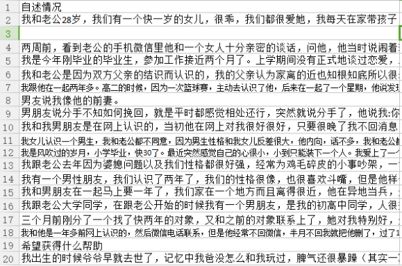
部分截图
接下来看看如何中文分词和去停用词操作,这两部分很基础的东西先讲,我之前有试过很多方式,觉得以下代码写法比较好(当然可能有更好的做法)
1.中文分词(jieba)和去停用词
分词用的是结巴分词,可以这样定义一个分词函数:
import jieba
mycut=lambda s:' '.join(jieba.cut(s))
下面案例中会介绍怎样用。
接下来看看去停用词,先是下载一个停用词表,导入到程序为stoplists变量(list类型),然后可以像下面操作:
import codecs
with codecs.open("stopwords.txt", "r", encoding="utf-8") as f:
    text = f.read()
stoplists=text.splitlines()
texts = [[word for word in document.split()if word not in stoplists] for document in documents]
  document变量在下面的LDA案例中会提到。
  接下来我根据LDA主题模型、Word2Vec实现、IF-IDF与词云的顺序进行案例的总结。
2.LDA主题模型案例
2.1导入相关库和数据
from gensim import corpora, models, similarities
import logging
import jieba
import pandas as pd

df = pd.read_csv('data.csv',encoding='gbk',header=None,sep="xovm02")
df= df[0] .dropna()  #[0]是因为我们的数据就是第一列,dropna去空
2.2分词处理
mycut=lambda s:' '.join(jieba.cut(s))
data=df[0].apply(mycut)
documents =data
2.3LDA模型计算(gensim)
# configuration 参数配置
logging.basicConfig(format='%(asctime)s : %(levelname)s : %(message)s', level=logging.INFO)
#去停用词处理
texts = [[word for word in document.split() if word not in stoplists] for document in documents]

# load id->word mapping (the dictionary) 单词映射成字典
dictionary = corpora.Dictionary(texts)

# word must appear >10 times, and no more than 40% documents
dictionary.filter_extremes(no_below=40, no_above=0.1)
# save dictionary
dictionary.save('dict_v1.dict')

# load corpus 加载语料库
corpus = [dictionary.doc2bow(text) for text in texts]

# initialize a model #使用TFIDF初始化
tfidf = models.TfidfModel(corpus)

# use the model to transform vectors, apply a transformation to a whole corpus 使用该模型来转换向量,对整个语料库进行转换
corpus_tfidf = tfidf[corpus]

# extract 100 LDA topics, using 1 pass and updating once every 1 chunk (10,000 documents), using 500 iterations
lda = models.LdaModel(corpus_tfidf, id2word=dictionary, num_topics=30, iterations=500)

# save model to files
lda.save('mylda_v1.pkl')

# print topics composition, and their scores, for the first document.
for index, score in sorted(lda[corpus_tfidf[0]], key=lambda tup: -1*tup[1]):
    print ("Score: {}\t Topic: {}".format(score, lda.print_topic(index, 5)))

# print the most contributing words for 100 randomly selected topics
lda.print_topics(30)

# print the most contributing words for 100 randomly selected topics
lda.print_topics(30)
应对不同情况就根据英语提示修改参数。
我在尝试的时候gensim的LDA函数还有另一个用法:
import gensim
#模型拟合,主题设为25
lda = gensim.models.ldamodel.LdaModel(corpus=corpus, id2word=dictionary, num_topics=25)

#打印25个主题,每个主题显示最高贡献的10个
lda.print_topics(num_topics=25, num_words=10)
3.Word2Vec案例(gensim)
为了简便,这里假设分词和去停用词已经弄好了。并保存为新的data.csv。
3.1导入相关库和文件
import pandas as pd
from gensim.models import Word2Vec
from gensim.models.word2vec import LineSentence

df = pd.read_csv('data.csv',encoding='gbk',header=None,sep="xovm02")
3.2开始Word2Vec的实现
sentences = df[0]
line_sent = []
for s in sentences:
    line_sent.append(s.split())  #句子组成list

model = Word2Vec(line_sent,
                 size=300,
                 window=5,
                 min_count=2,
                 workers=2)      #word2vec主函数(API)

model.save('./word2vec.model')
print(model.wv.vocab)  #vocab是个字典类型
print (model.wv['分手']) #打印“分手”这个词的向量

model.similarity(u"分手", u"爱情")#计算两个词之间的余弦距离
model.most_similar(u"分手")#计算余弦距离最接近“分手”的10个词
4.TF-IDF的计算和词云
4.1TF-IDF的计算
如果需要计算文本的TF-IDF值,可以参考下面操作:
#导入sklearn相关库
from sklearn.feature_extraction.text import TfidfTransformer
from sklearn.feature_extraction.text import CountVectorizer

vectorizer=CountVectorizer()
transformer=TfidfTransformer()

#计算TF-IDF值(data是你自己的文本数据)
#这一个是主函数
tfidf=transformer.fit_transform(vectorizer.fit_transform(data))
weight=tfidf.toarray()

#后续需要:
#选出的单词结果
words=vectorizer.get_feature_names()
#得到词频
vectorizer.fit_transform(data)
4.2词云
from scipy.misc import imread
import matplotlib.pyplot as plt
from wordcloud import WordCloud, ImageColorGenerator

font_path = 'E:\simkai.ttf' # 为matplotlib设置中文字体路径没

#词云主函数
# 设置词云属性
wc = WordCloud(font_path=font_path,  # 设置字体
               background_color="white",  # 背景颜色
               max_words=200,  # 词云显示的最大词数
               #mask=back_coloring,  # 设置背景图片
               max_font_size=200,  # 字体最大值
               random_state=42,
               width=1000, height=860, margin=2,# 设置图片默认的大小,但是如果使用背景图片的话,那么保存的图片大小将会按照其大小保存,margin为词语边缘距离
               )
#词云计算(假设data为你处理好需要做词云的文本数据)
wc.generate(data)

plt.figure()
# 以下代码显示图片
plt.imshow(wc)
plt.axis("off")
plt.show()
# 绘制词云

#将结果保存到当前文件夹
from os import path
d = path.dirname('.')
wc.to_file(path.join(d, "词云.png"))
5.结语
以上就是我在实践过程中使用的处理文本的一些方法,当然肯定有比这些更好的方法。
写的比较匆忙,我想等我放假再把里面不够详细的地方补全。
这一次的学习经历大约到这里就要结束了,后面就是不断总结补充和改进。