吴恩达机器学习作业1- 线性回归作业(python实现)
机器学习练习1 python复现- 线性回归
单变量线性回归
import numpy as np
import pandas as pd
import matplotlib.pyplot as plt
path = 'ex1data1.txt'
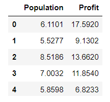
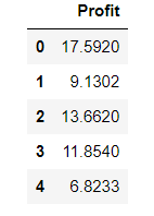
data = pd.read_csv(path, header=None, names=['Population', 'Profit'])
data.head()
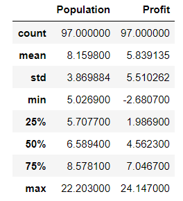
data.describe()
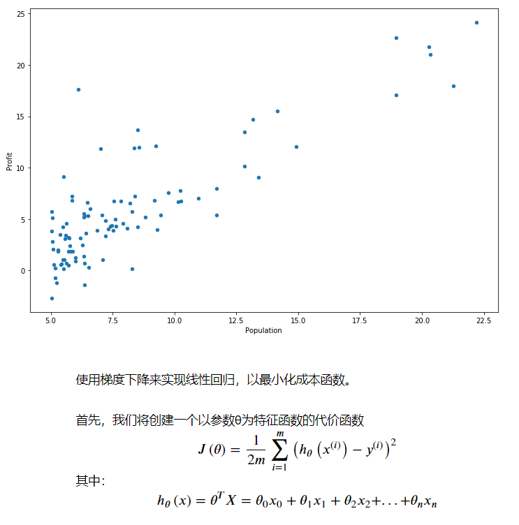
看下数据长什么样子
data.plot(kind='scatter', x='Population', y='Profit', figsize=(12,8))
plt.show()
def computeCost(X, y, theta):
    inner = np.power(((X * theta.T) - y), 2)
    return np.sum(inner) / (2 * len(X))
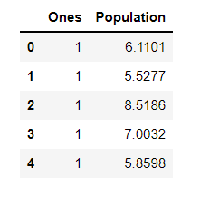
让我们在训练集中添加一列,以便我们可以使用向量化的解决方案来计算代价和梯度。
data.insert(0, 'Ones', 1)
现在我们来做一些变量初始化。
# set X (training data) and y (target variable)
cols = data.shape[1]
X = data.iloc[:,0:cols-1]#X是所有行,去掉最后一列
y = data.iloc[:,cols-1:cols]#X是所有行,最后一列
观察下 X (训练集) and y (目标变量)是否正确.
X.head()#head()是观察前5行
y.head()
代价函数是应该是numpy矩阵,所以我们需要转换X和Y,然后才能使用它们。 我们还需要初始化theta。
#使得numpy得到的数组矩阵化
X = np.matrix(X.values)
y = np.matrix(y.values)
theta = np.matrix(np.array([0,0]))
theta 是一个(1,2)矩阵
theta
matrix([[0, 0]])
看下维度
X.shape, theta.shape, y.shape
((97, 2), (1, 2), (97, 1))
计算代价函数 (theta初始值为0).
computeCost(X, y, theta)
32.072733877455676
batch gradient decent(批量梯度下降)
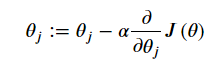
def gradientDescent(X, y, theta, alpha, iters):
    temp = np.matrix(np.zeros(theta.shape))
    #ravel使多维矩阵降为一维,获取得到相应矩阵元素的个数
    parameters = int(theta.ravel().shape[1])
    cost = np.zeros(iters)

    for i in range(iters):
        error = (X * theta.T) - y

        for j in range(parameters):
            term = np.multiply(error, X[:,j])
            temp[0,j] = theta[0,j] - ((alpha / len(X)) * np.sum(term))

        theta = temp
        cost[i] = computeCost(X, y, theta)

    return theta, cost
初始化一些附加变量 - 学习速率α和要执行的迭代次数。
alpha = 0.01
iters = 1000
现在让我们运行梯度下降算法来将我们的参数θ适合于训练集。
g, cost = gradientDescent(X, y, theta, alpha, iters)
g
matrix([[-3.24140214, 1.1272942 ]])
最后,我们可以使用我们拟合的参数计算训练模型的代价函数(误差)。
computeCost(X, y, g)
4.5159555030789118
现在我们来绘制线性模型以及数据,直观地看出它的拟合。
x = np.linspace(data.Population.min(), data.Population.max(), 100)
f = g[0, 0] + (g[0, 1] * x)

fig, ax = plt.subplots(figsize=(12,8))
ax.plot(x, f, 'r', label='Prediction')
ax.scatter(data.Population, data.Profit, label='Traning Data')
ax.legend(loc=2)
ax.set_xlabel('Population')
ax.set_ylabel('Profit')
ax.set_title('Predicted Profit vs. Population Size')
plt.show()

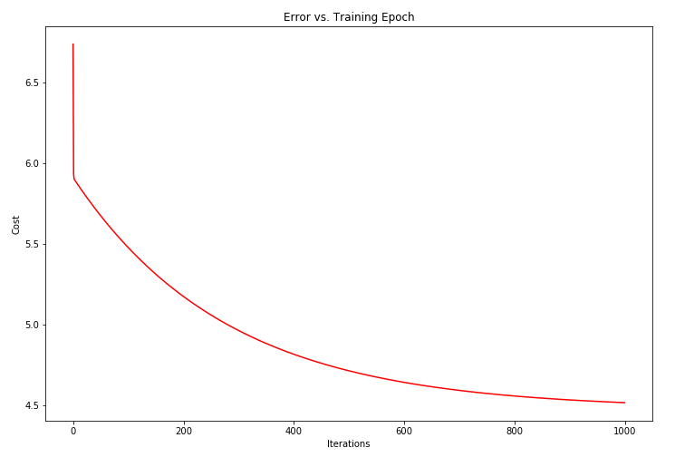
由于梯度方程式函数也在每个训练迭代中输出一个代价的向量,所以我们也可以绘制。 请注意,代价总是降低 - 这是凸优化问题的一个例子。
fig, ax = plt.subplots(figsize=(12,8))
ax.plot(np.arange(iters), cost, 'r')
ax.set_xlabel('Iterations')
ax.set_ylabel('Cost')
ax.set_title('Error vs. Training Epoch')
plt.show()
多变量线性回归
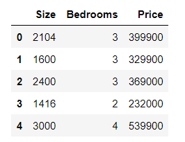
练习1还包括一个房屋价格数据集,其中有2个变量(房子的大小,卧室的数量)和目标(房子的价格)。 我们使用我们已经应用的技术来分析数据集。
path =  'ex1data2.txt'
data2 = pd.read_csv(path, header=None, names=['Size', 'Bedrooms', 'Price'])
data2.head()
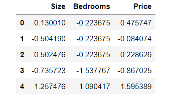
对于此任务,我们添加了另一个预处理步骤 - 特征归一化。 这个对于pandas来说很简单
data2 = (data2 - data2.mean()) / data2.std()
data2.head()
现在我们重复第1部分的预处理步骤,并对新数据集运行线性回归程序。
# add ones column
data2.insert(0, 'Ones', 1)

# set X (training data) and y (target variable)
cols = data2.shape[1]
X2 = data2.iloc[:,0:cols-1]
y2 = data2.iloc[:,cols-1:cols]

# convert to matrices and initialize theta
X2 = np.matrix(X2.values)
y2 = np.matrix(y2.values)
theta2 = np.matrix(np.array([0,0,0]))

# perform linear regression on the data set
g2, cost2 = gradientDescent(X2, y2, theta2, alpha, iters)

# get the cost (error) of the model
computeCost(X2, y2, g2)
0.13070336960771892
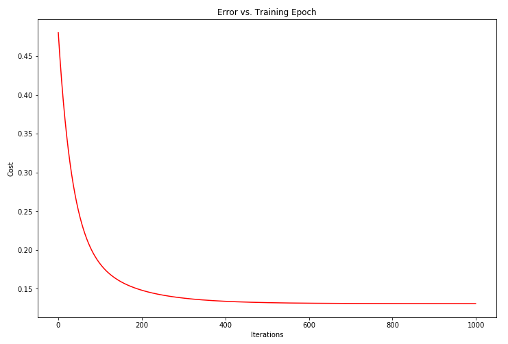
我们也可以快速查看这一个的训练进程。
fig, ax = plt.subplots(figsize=(12,8))
ax.plot(np.arange(iters), cost2, 'r')
ax.set_xlabel('Iterations')
ax.set_ylabel('Cost')
ax.set_title('Error vs. Training Epoch')
plt.show()
我们也可以使用scikit-learn的线性回归函数,而不是从头开始实现这些算法。 我们将scikit-learn的线性回归算法应用于第1部分的数据,并看看它的表现。
from sklearn import linear_model
model = linear_model.LinearRegression()
model.fit(X, y)
LinearRegression(copy_X=True, fit_intercept=True, n_jobs=1, normalize=False)
scikit-learn model的预测表现
x = np.array(X[:, 1].A1)
f = model.predict(X).flatten()

fig, ax = plt.subplots(figsize=(12,8))
ax.plot(x, f, 'r', label='Prediction')
ax.scatter(data.Population, data.Profit, label='Traning Data')
ax.legend(loc=2)
ax.set_xlabel('Population')
ax.set_ylabel('Profit')
ax.set_title('Predicted Profit vs. Population Size')
plt.show()

4. normal equation(正规方程)
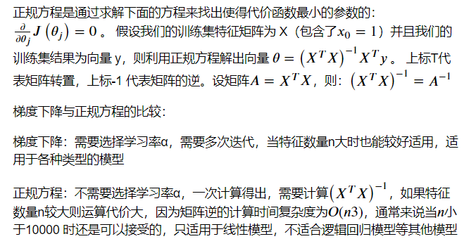
# 正规方程
def normalEqn(X,y):
    #linalg.inv表示求逆
    theta = np.linalg.inv(X.T.dot(X)).dot(X.T.dot(y))
    return theta
final_theta2=normalEqn(X, y)#感觉和批量梯度下降的theta的值有点差距
final_theta2
matrix([[-3.89578088],
        [ 1.19303364]])
梯度下降得到的结果是matrix([[-3.24140214, 1.1272942 ]])
