
幅度分布-分类器(无线信道模型)(原创)
幅度分布-分类器(无线信道模型)
遇到问题:
1,瑞丽信道和莱斯信道重合度较高
2,对数正态信道的波形失真严重
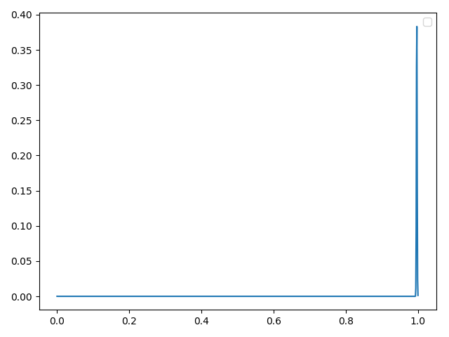
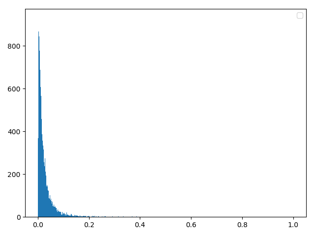
一,平坦分布(经检验正确)
方法一:理论合成
mean = np.random.uniform(0.5, 2, 1)
data = np.random.normal(mean, 0.001, sampleNo)
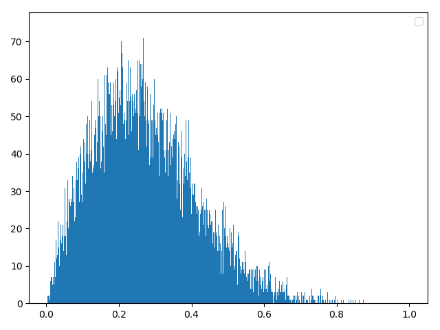
二,瑞利分布(三种方法任选其一即可)
# 方法一:理论合成
delta = 2
data0 = np.random.normal(0, delta, 20000)
data1 = np.random.normal(0, delta, 20000)
data = (data0**2+data1**2)**0.5
方法二:反函数构建
data0 = np.random.random(20000)
data = 2 * np.sqrt(-2 * np.log(data0))
方法三:numpy自带库
scale = np.random.normal(loc=0.0, scale=20)
d0 = np.random.rayleigh(abs(scale), 40000)
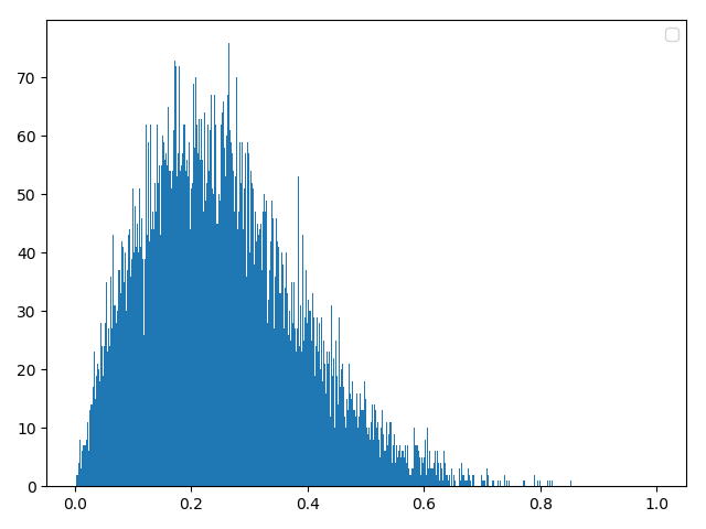
三,莱斯分布
方法一:理论合成(经确认,这个理论是正确的)
data0 = np.random.normal(loc=0.0, scale=1, size=length)
data1 = np.random.normal(loc=0.0, scale=1, size=length)
data = np.sqrt((data0 + a) ** 2 + data1 ** 2)

方法二:反函数(这个方法问题很大)(经检验这个是属于对数正态分布的推导)
data0 = np.random.normal(loc=0.0, scale=abs(delta), size=length)
data = np.exp(u + delta * data0)
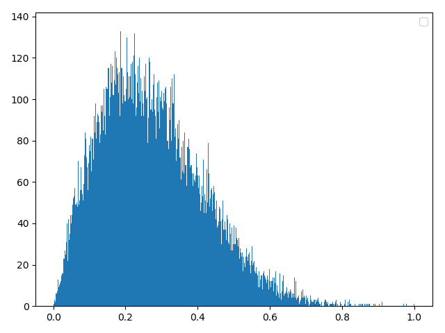
四,对数正态分布
方法一:理论合成(与瑞利信道的反函数雷同!!!)(经检验完全正确)
data1 = np.random.normal(0, 1, sampleNo )
data = np.exp(u+delta*data1)
方法二:公式法(和理想差距较大,原因:数据量没有达到一定程度。舍弃)
for i in range(len(x)):
if Y[i] <= lognormal(x[i],u,delta):
data.append(x[i])
方法三:numpy自带库(numpy自带库和理论合成效果相同)
d0 = np.random.lognormal(mean, sigma, 40000)
五,Suzuki分布(确认正确)
方法一:理论合成
data0 = np.random.normal(0, 1, sampleNo)
data1 = np.random.normal(0, 1, sampleNo)
data3 = np.random.normal(0, 1, sampleNo)
u = np.sqrt(data0**2+data1**2)
v = np.exp(m+s*data3)
data = u*v
六,引入数据预处理
均值:一阶中心矩
方差:二阶中心矩
中位数:数值从大到小(或者反序)最中间的数值
众数:出现频次最高的数值(这两个数据需要额外处理)
偏度:统计数据分布非对称程度的数字特征
峰度:表征概率密度分布曲线在平均值处峰值高低的特征数
平均绝对误差:所有单个观测值与算术平均值的偏差的绝对值的平均
与此同时遇到了一个新的问题:
这些数据处理方法使用原始数据还是统计数据!
个人更倾向于统计数据,因为原始数据太过庞大并且数据格式不固定得出来的样值不具有代表性(打脸,统计数据无法使用)
统计数据无法使用的原因:因为上面的数据预处理本身就是一个统计的过程,如果使用统计数据那就相当于 原始数据→统计1→统计2,统计两次!
原始数据的改进:1,样本量的减小(但是分布函数依旧);2,将原始数据的预处理数据进行打包减少数据量;3,数据格式直接使用全局的统计即可(这个有可能会出现问题)
实际计算过程中的错误:众数无法使用;原因:这个是float64精度的几乎没有相等的两个数值
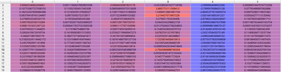
数据预处理:(列为样本序号,横轴依次为均值、标准差、中位数、偏度、峰度、平均绝对误差)
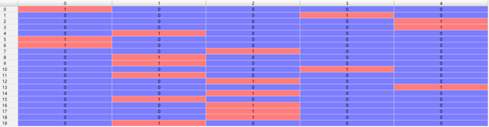
原始数据标签:(列为样本序号,横轴依次为平坦分布、瑞利分布、莱斯分布、对数正态分布、suzuki分布)
七,分类器设计
由之前做FashionAI的服饰标签属性时设计的CNN训练模型,现在直接拿来改版一下当幅度分布分类器的训练模型(改成DNN网络即可)
1,DNN结构
# local1 全连接层 1 [6,128]
# local2 全连接层 2 [128,512]
# local3 全连接层 3 [512,128]
# softmax 全连接层 4 [128,5]
BATCH_SIZE = 256
CAPACITY = 128
learn_rate = 0.0010485759
step_damp = 100
rate_damp = 0.9
MAX_STEP = 160000
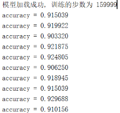
2,训练效果
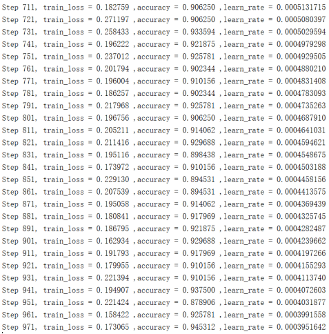
通过上图可知正确率在91%左右,其中为什么不能达到100%的原因,这个是因为:
① 莱斯分布在主径分量接近零的时候会退化成瑞利分布;
② suzuki分布和对数正态的相似性较大;
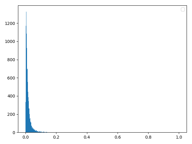
模拟数据验证1:(Batch_size=64)
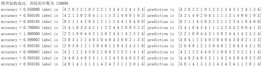
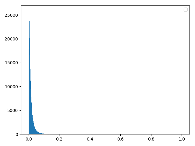
模拟数据验证2:(Batch_size=1024)
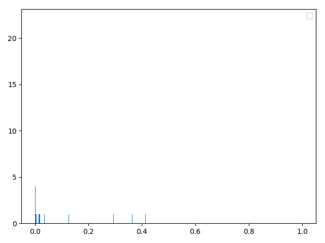
3,实测数据检验
八,总结
其实这个 幅度分布-分类器 更难设计
难点:
①这个是对个分布函数的随机数数据
②处理数据比较麻烦,直接把随机数的输出输入分类器效果基本为0,这个思路问题很大,并且计算量还大
③统计数据后进行数据预处理,在这里也出现了相关的问题,比如上文说的统计两次的错误
④分类器模型设计,之前都是使用图像处理的卷积网络,由于惯性的缘故。刚开始也想使用一维卷积网络,但是效果一般
附录代码:input.pyw
  1 # coding=utf-8
  2 # coded by Mufasa 2018.12.10
  3 # 数据生成程序
  4 # 程序说明:整个体系的数据来源 version3.1
  5 #
  6 """
  7 改进:
  8 ① 将所有的数据进行,再次的验证,舍弃不合理的,提取正确的数据
  9 ② 将与处理数据引入,例如:均值、方差、中位数、众数、峰度、偏度、平均绝对误差
 10 ③ 数据打包测试完成
 11 输出:
 12 d1_batch                [BATCH_SIZE,6]
 13 np.array(d2_batch)      [BATCH_SIZE]
 14 """
 15
 16 import numpy as np
 17
 18
 19 class data_deal:
 20     def d_mean(self, data):  # 均值
 21         return np.mean(data)
 22
 23     def d_var(self, data):  # 方差
 24         return np.var(data)
 25
 26     def d_med(self, data):  # 中位数
 27         return np.median(data)
 28
 29     def d_mod(self, data):  # 众数
 30         counts = np.bincount(data)
 31         return np.argmax(counts)
 32
 33     def d_kur(self, data):  # 峰度
 34         n = len(data)
 35         mean = np.mean(data)
 36         sigma = np.var(data)
 37         niu4_u = sum((data - mean) ** 4) / n
 38         return niu4_u / (sigma ** 2) - 3
 39
 40     def d_par(self, data):  # 偏度
 41         n = len(data)
 42         mean = np.mean(data)
 43         sigma = np.cov(data)
 44         niu3_0 = data ** 3 / n
 45         return (niu3_0 - 3 * mean * sigma ** 2 - mean ** 3) / (sigma ** 3)
 46
 47     def d_mea_abs_err(self, data):  # 平均绝对误差
 48         n = len(data)
 49         mean = np.mean(data)
 50         return sum(abs(data - mean)) / n
 51
 52     def out_all(self, data):
 53         n = len(data)
 54         niu = sum(data) / n  # 均值
 55         niu2 = sum(data ** 2) / n
 56         niu3 = sum(data ** 3) / n  # 三阶原点矩
 57
 58         sigma2 = niu2 - niu * niu  # 方差
 59         sigma = np.sqrt(sigma2)  # 标准差
 60         median = np.median(data)  # 中位数
 61
 62         skewness = (niu3 - 3 * niu * sigma2 - niu ** 3) / (sigma ** 3)  # 偏度
 63         niu4_u = sum((data - niu) ** 4) / n  # 四阶中心矩
 64         kurtosis = niu4_u / (sigma ** 2) - 3  # 峰度
 65         mea_abs_err = sum(abs(data - niu)) / n  # 平均绝对误差
 66         return [niu, sigma, median, skewness, kurtosis, mea_abs_err]
 67
 68
 69 # 整合 5种数据生成、数据标签、数据保存
 70 class data_origin:
 71     def __init__(self, sampleNo):
 72         self.sampleNo = sampleNo  # 随机幅度样本个数
 73         # self.bins = bins  # 样本统计切片个数
 74         self.fun = {
 75             0: self.impulse,
 76             1: self.rayleigh,
 77             2: self.rice,
 78             3: self.lognormal,
 79             4: self.suzuki}
 80
 81     def data_sum(self, num):
 82         d2_batch = []
 83         for i in range(num):
 84             select = np.random.randint(0, 5)
 85             fun_now = self.fun[select]
 86             data, d2 = fun_now()
 87             d1 = data_deal.out_all(self, data)
 88             d2_batch.append(d2)
 89             if i == 0:
 90                 d1_batch = d1
 91             else:
 92                 d1_batch = np.vstack((d1_batch, d1))
 93         return d1_batch, np.array(d2_batch)
 94
 95     # 第一个 冲激分布  [1 0 0 0 0] 理论上完全正确
 96     def impulse(self):  # 测试正确
 97         mean = np.random.uniform(0.5, 2, 1)
 98
 99         data = np.random.normal(mean, 0.001, self.sampleNo)
100         data = data / max(data)  # 数据归一化处理
101
102         d2 = 0
103         return data, d2
104
105     # 第二个 瑞利分布  [0 1 0 0 0]
106     def rayleigh(self):  # 使用理论生成数据(双高斯信号),测试正确
107         sigma = np.random.normal(2, 1, 1)[0]
108
109         data0 = np.random.normal(loc=0.0, scale=abs(sigma), size=self.sampleNo)
110         data1 = np.random.normal(loc=0.0, scale=abs(sigma), size=self.sampleNo)
111         data = np.sqrt((data0 ** 2 + data1 ** 2))
112         data = data / max(data)  # 数据归一化处理
113
114         d2 = 1
115         return data, d2
116
117     # 第三个 莱斯分布  [0 0 1 0 0]
118     def rice(self):  # 测试正确
119         k = np.random.uniform(0, 15)
120         mean = np.sqrt(2 * k)
121
122         data0 = np.random.normal(loc=0.0, scale=1, size=self.sampleNo)
123         data1 = np.random.normal(loc=0.0, scale=1, size=self.sampleNo)
124
125         data = np.sqrt((data0 + mean) ** 2 + data1 ** 2)
126         data = data / max(data)  # 数据归一化处理
127
128         d2 = 2
129         return data, d2
130
131     # 第四个 对数正态分布  [0 0 0 1 0]
132     def lognormal(self):
133         u = 0  # 这里的u值可以通过归一化清除
134         delta = np.random.uniform(1 / 2, 1)  # delta的取值才是对数正态的核心
135
136         data0 = np.random.normal(loc=0.0, scale=delta, size=self.sampleNo)
137         data = np.exp(u + delta * data0)
138         data = data / max(data)
139
140         d2 = 3
141         return data, d2
142
143     # 第五个 Suzuki分布  [0 0 0 0 1]
144     def suzuki(self):
145         m = np.random.normal(0, 1, 1)[0]  # 这里的sigma数值需要查数据,看看sigma的取值规律
146         s = np.random.uniform(0.3, 0.8)  # 这里的sigma数值需要查数据,看看sigma的取值规律
147
148         data0 = np.random.normal(loc=0.0, scale=1, size=self.sampleNo)
149         data1 = np.random.normal(loc=0.0, scale=1, size=self.sampleNo)
150         data2 = np.random.normal(loc=0.0, scale=1, size=self.sampleNo)
151         u = np.sqrt(data0 ** 2 + data1 ** 2)
152         v = np.exp(m + s * data2)
153         data = u * v
154         data = data / max(data)
155
156         d2 = 4
157         return data, d2
158
159
160 # 测试
161 # obj = data_origin(700, 1000)
162 # d1, d2 = obj.data_sum(20)
163 # d1, d2 = obj.impulse()
164 # print(d1)
165 # print(d1[19, 1])  # [batch_size,num]
166 # print(d2)
167 # show_ = show()
168 # print(d1)
169 # show_.broken_line(np.array(range(0, 1000)), d1)
170 # pass
附录代码:model.pyw
 1 # coding=utf-8
 2
 3
 4 # local1 全连接层 1     [6,128]
 5 # local2 全连接层 2     [128,512]
 6 # local3 全连接层 3     [512,128]
 7 # softmax 全连接层 4    [128,5]
 8
 9
10 import tensorflow as tf
11
12
13 def inference(images, batch_size, n_classes):
14     with tf.variable_scope('local1') as scope:
15         # reshape = tf.reshape(images, shape=[batch_size, -1])
16         # dim = reshape.get_shape()[1].value
17         # print(dim)
18         weights = tf.get_variable('weights',
19                                   shape=[6, 128],
20                                   dtype=tf.float32,
21                                   initializer=tf.truncated_normal_initializer(stddev=0.005, dtype=tf.float32))
22         biases = tf.get_variable('biases',
23                                  shape=[128],
24                                  dtype=tf.float32,
25                                  initializer=tf.constant_initializer(0.1))
26     local1 = tf.nn.relu(tf.matmul(images, weights) + biases, name=scope.name)
27
28     # local2
29     with tf.variable_scope('local2') as scope:
30         weights = tf.get_variable('weights',
31                                   shape=[128, 512],
32                                   dtype=tf.float32,
33                                   initializer=tf.truncated_normal_initializer(stddev=0.005, dtype=tf.float32))
34         biases = tf.get_variable('biases',
35                                  shape=[512],
36                                  dtype=tf.float32,
37                                  initializer=tf.constant_initializer(0.1))
38         local2 = tf.nn.relu(tf.matmul(local1, weights) + biases, name='local4')
39
40     # local3
41     with tf.variable_scope('local3') as scope:
42         weights = tf.get_variable('weights',
43                                   shape=[512, 128],
44                                   dtype=tf.float32,
45                                   initializer=tf.truncated_normal_initializer(stddev=0.005, dtype=tf.float32))
46         biases = tf.get_variable('biases',
47                                   shape=[128],
48                                   dtype=tf.float32,
49                                   initializer=tf.constant_initializer(0.1))
50         local3 = tf.nn.relu(tf.matmul(local2, weights) + biases, name='local4')
51
52         # softmax
53     with tf.variable_scope('softmax_linear') as scope:
54         weights = tf.get_variable('softmax_linear',
55                                   shape=[128, n_classes],
56                                   dtype=tf.float32,
57                                   initializer=tf.truncated_normal_initializer(stddev=0.005, dtype=tf.float32))
58         biases = tf.get_variable('biases',
59                                  shape=[n_classes],
60                                  dtype=tf.float32,
61                                  initializer=tf.constant_initializer(0.1))
62         softmax_linear = tf.add(tf.matmul(local3, weights), biases, name='softmax_linear')
63
64     return softmax_linear
65
66
67 def losses(logits, labels):
68     with tf.variable_scope('loss') as scope:
69         cross_entropy = tf.nn.sparse_softmax_cross_entropy_with_logits \
70             (logits=logits, labels=labels, name='xentropy_per_example')
71         loss = tf.reduce_mean(cross_entropy, name='loss')
72         tf.summary.scalar(scope.name + '/loss', loss)
73     return loss
74
75
76 def trainning(loss, learning_rate, global_step):
77     # with tf.name_scope('optimizer'):
78     with tf.variable_scope('optimizer') as scope:
79         optimizer = tf.train.AdamOptimizer(learning_rate=learning_rate)
80         # global_step = tf.Variable(0, name='global_step', trainable=False)
81         train_op = optimizer.minimize(loss, global_step=global_step)
82     return train_op
83
84
85 def evaluation(logits, labels):
86     with tf.variable_scope('accuracy') as scope:
87         correct = tf.nn.in_top_k(logits, labels, 1)
88         correct = tf.cast(correct, tf.float16)
89         accuracy = tf.reduce_mean(correct)
90         tf.summary.scalar(scope.name + '/accuracy', accuracy)
91     return accuracy
附录代码:train.pyw
 1 # coding=utf-8
 2 # 产生数据—训练-评估-结束标准
 3 # 这里使用的数据是随机生成的,理论上是穷举数据集,评估和训练本质上一致的
 4 '''
 5 改进:
 6 ① 将保存的训练参数使用相对路径
 7
 8 '''
 9
10 import input
11 import model
12 import numpy as np
13 import os
14 import tensorflow as tf
15
16 bins = 6
17 sum_num = 1000
18 n_classes = 5
19
20 BATCH_SIZE = 256
21 CAPACITY = 128
22 learn_rate = 0.0010485759
23 step_damp = 100
24 rate_damp = 0.9
25 MAX_STEP = 160000
26
27 root_folder = os.path.dirname(os.path.realpath(__file__))
28 os.chdir(root_folder)  # 返回上一级文件夹
29 # print(root_folder)
30 # print(os.path.dirname(root_folder))
31 folder = "model2//"  # 使用相对路径
32 obj = input.data_origin(sum_num)
33 '''
34 DNN配置
35 '''
36 os.environ["CUDA_VISIBLE_DEVICES"] = '0'  # 指定第一块GPU可用
37 config = tf.ConfigProto(allow_soft_placement=True)
38 config.gpu_options.per_process_gpu_memory_fraction = 0.85  # 程序最多只能占用指定gpu 70%的显存
39 config.gpu_options.allow_growth = True  # 程序按需申请内存
40 with tf.Session(config=config) as sess:
41     global_step = tf.Variable(0, name='global_step', trainable=False)  # 有变更,需要注意
42     learning_rate = tf.train.exponential_decay(learn_rate, global_step, step_damp, rate_damp, staircase=False)
43
44     data_batch = tf.placeholder(dtype=tf.float32, shape=[BATCH_SIZE, bins], name='data')
45     label_batch = tf.placeholder(dtype=tf.int32, shape=[BATCH_SIZE], name='label')
46
47     train_logits = model.inference(data_batch, BATCH_SIZE, n_classes)
48     train_loss = model.losses(train_logits, label_batch)
49     train_op = model.trainning(train_loss, learning_rate, global_step)
50     train__acc = model.evaluation(train_logits, label_batch)
51
52     summary_op = tf.summary.merge_all()
53     train_writer = tf.summary.FileWriter(folder, sess.graph)
54     saver = tf.train.Saver()
55
56     sess.run(tf.global_variables_initializer())
57     for step in np.arange(MAX_STEP):
58         data, label = obj.data_sum(BATCH_SIZE)
59         _ = sess.run(train_op, {data_batch: data, label_batch: label})
60         if step % step_damp == 0:
61             step_now, tra_loss, learn_rate, accuracy_now = sess.run(
62                 [global_step, train_loss, learning_rate, train__acc], {data_batch: data, label_batch: label})
63
64             print('Step %d, train_loss = %f ,accuracy = %f ,learn_rate = %.10f ' % (
65             step_now, tra_loss, accuracy_now, learn_rate))
66         if (step % 10000 == 0) or ((step + 1) == MAX_STEP):
67             checkpoint_path = os.path.join(folder, 'model.ckpt')
68             saver.save(sess, checkpoint_path, global_step=step)
附录代码:evaluate.pyw
 1 # coding=utf-8
 2 # 产生数据—训练-评估-结束标准
 3 # 这里使用的数据是随机生成的,理论上是穷举数据集,评估和训练本质上一致的
 4 """
 5 改进:
 6 ① 将保存的训练参数使用相对路径
 7
 8 """
 9
10 import input
11 import model
12 import numpy as np
13 import os
14 import tensorflow as tf
15
16 bins = 6
17 sum_num = 1000
18 n_classes = 5
19
20 BATCH_SIZE = 2048
21 CAPACITY = 128
22 step = 10
23
24 root_folder = os.path.dirname(os.path.realpath(__file__))
25 os.chdir(root_folder)  # 返回上一级文件夹
26
27 logs_train_dir = "model2"  # 使用相对路径
28 obj = input.data_origin(sum_num)
29
30
31 def evaluate(logs_train_dir, BATCH_SIZE):
32     # GPU计算资源参数
33     os.environ["CUDA_VISIBLE_DEVICES"] = '0'  # 指定第一块GPU可用
34     config = tf.ConfigProto(allow_soft_placement=True)
35     config.gpu_options.per_process_gpu_memory_fraction = 0.85  # 程序最多只能占用指定gpu 70%的显存
36     config.gpu_options.allow_growth = True  # 程序按需申请内存
37     with tf.Session(config=config) as sess:
38
39         data_batch = tf.placeholder(dtype=tf.float32, shape=[BATCH_SIZE, bins], name='data')
40         label_batch = tf.placeholder(dtype=tf.int32, shape=[BATCH_SIZE], name='label')
41
42         train_logits = model.inference(data_batch, BATCH_SIZE, n_classes)
43         # evaluate_logits = tf.nn.softmax(train_logits)
44         evaluate_logits = tf.argmax(train_logits, 1)
45         train__acc = model.evaluation(train_logits, label_batch)
46
47         # 计算图保存参数
48         # summary_op = tf.summary.merge_all()
49         # train_writer = tf.summary.FileWriter(logs_train_dir, sess.graph)
50         saver = tf.train.Saver()
51
52         sess.run(tf.global_variables_initializer())
53         # coord = tf.train.Coordinator()
54         # threads = tf.train.start_queue_runners(sess=sess, coord=coord)
55
56         # 加载训练后的参数
57         ckpt = tf.train.get_checkpoint_state(logs_train_dir)
58         if ckpt and ckpt.model_checkpoint_path:
59             global_step = ckpt.model_checkpoint_path.split('/')[-1].split('-')[-1]
60             saver.restore(sess, ckpt.model_checkpoint_path)
61             print('模型加载成功, 训练的步数为 %s' % global_step)
62         else:
63             print('模型加载失败,,,文件没有找到')
64
65         # 写入预测数据前期设置
66         try:
67             for i in np.arange(step):
68                 data, label = obj.data_sum(BATCH_SIZE)
69                 # if coord.should_stop():
70                 #     break
71                 # accuracy_now, prediction = sess.run([train__acc, evaluate_logits],
72                 #                                     {data_batch: data, label_batch: label})
73                 # print('accuracy = %f' % (accuracy_now), 'label is ', label, 'prediction is ', prediction)
74
75                 accuracy_now = sess.run(train__acc,{data_batch: data, label_batch: label})
76                 print('accuracy = %f' % accuracy_now)
77
78         except tf.errors.OutOfRangeError:
79             print('Done training -- epoch limit reached')
80         # finally:
81         #     coord.request_stop()
82         # coord.join(threads)
83         # print("正常预测第", circle, "个数据", label[circle])
84     sess.close()
85
86
87 evaluate(logs_train_dir, BATCH_SIZE)

