触发字检测 trigger word detection
触发字检测 trigger word detection
欢迎来到这个专业的最终编程任务!
在本周的视频中,您学习了如何将深度学习应用于语音识别。在此任务中,您将构建语音数据集并实现触发词检测算法(有时也称为关键字检测或唤醒字检测)。触发词检测技术允许Amazon Alexa,Google Home,Apple Siri和Baidu DuerOS 等设备听到某个单词后唤醒。
对于本练习,我们的触发词将是“Activate”。每次听到你说“Activate”,它都会发出“chiming”的声音。在此作业结束时,您将能够录制自己说话的片段,并在检测到您说“activate”时让算法触发铃声。
完成此任务后,您也可以将其扩展为在笔记本电脑上运行,这样每次您说“激活”它都会启动您喜欢的应用程序,或打开您家中的网络连接灯,或触发其他一些事件?
在此作业中,您将学习:
- 构建语音识别项目
- 合成和处理录音以创建训练/开发数据集
- 训练触发词检测模型并进行预测
让我们开始吧!运行以下单元格以加载要使用的包。
import numpy as np
from pydub import AudioSegment #需要安装ffmpeg
import random
import sys
import io
import os
import glob
import IPython
from td_utils import *
%matplotlib inline
1 - 数据合成:创建语音数据集
让我们首先为触发词检测算法构建数据集。理想情况下,语音数据集应尽可在您要运行它的应用程序的地方采集。在这种情况下,您希望在工作环境(图书馆,家庭,办公室,开放空间......)中检测“activate”一词。因此,您需要在不同的背景声音上创建正面词(“activate”)和负面词(除激活之外的随机词)的混合录音。我们来看看如何创建这样的数据集。
1.1 - 听取数据
你的一个朋友正在帮助你完成这个项目,他们去了该地区的图书馆,咖啡馆,餐馆,家庭和办公室,以记录背景噪音,以及人们说正面/负面词语的音频片段。该数据集包括以各种说话口音的人。
在raw_data目录中,您可以找到正面单词,负面单词和背景噪音的原始音频文件的子集。您将使用这些音频文件来合成数据集以训练模型。 “activate”目录包含人们说“activate”一词的正面例子。 “negatives”目录包含人们说“activate”以外的随机词的负面例子。每个录音有一个单词。 “backgrounds”目录包含10s的不同环境中的背景噪声剪辑。
运行下面的单元格以听取一些示例。
IPython.display.Audio("./raw_data/activates/1.wav")
IPython.display.Audio("./raw_data/negatives/4.wav")
IPython.display.Audio("./raw_data/backgrounds/1.wav")
您将使用这三种类型的记录(正/负/背景)来创建标记数据集 labelled dataset。
1.2 - 从录音到频谱图
什么是录音?麦克风记录的空气压力随时间变化很小,正是这些气压的微小变化使您的耳朵也感觉到声音。您可以认为录音是一长串数字,用于测量麦克风检测到的微小气压变化。我们将使用44100 Hz(或44100Hertz)的音频采样。这意味着麦克风每秒给我们44100个数字。因此,10秒音频剪辑由441000个数字表示(= \(10 \times 44100\))。
很难从音频的这种“"raw" representation audio中找出“activate”这个词是否被说出来。为了帮助您的序列模型更容易学习检测触发词,我们将计算音频的谱图spectrogram 。频谱图告诉我们在某个时刻音频片段中存在多少不同的频率。
(如果你曾经进行过信号处理或傅立叶变换的高级课程,则通过在原始音频信号上滑动窗口来计算频谱图,并使用傅里叶变换计算每个窗口中最活跃的频率。如果不理解上一句话,不用担心。)
让我们看一个例子。
IPython.display.Audio("audio_examples/example_train.wav")
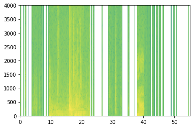
x = graph_spectrogram("audio_examples/example_train.wav")
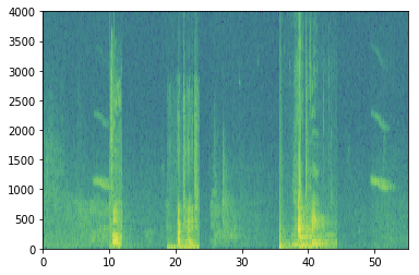
上图表示了在多个时间步长(x轴)上每个频率(y轴)的活动程度。
The graph above represents how active each frequency is (y axis) over a number of time-steps (x axis).
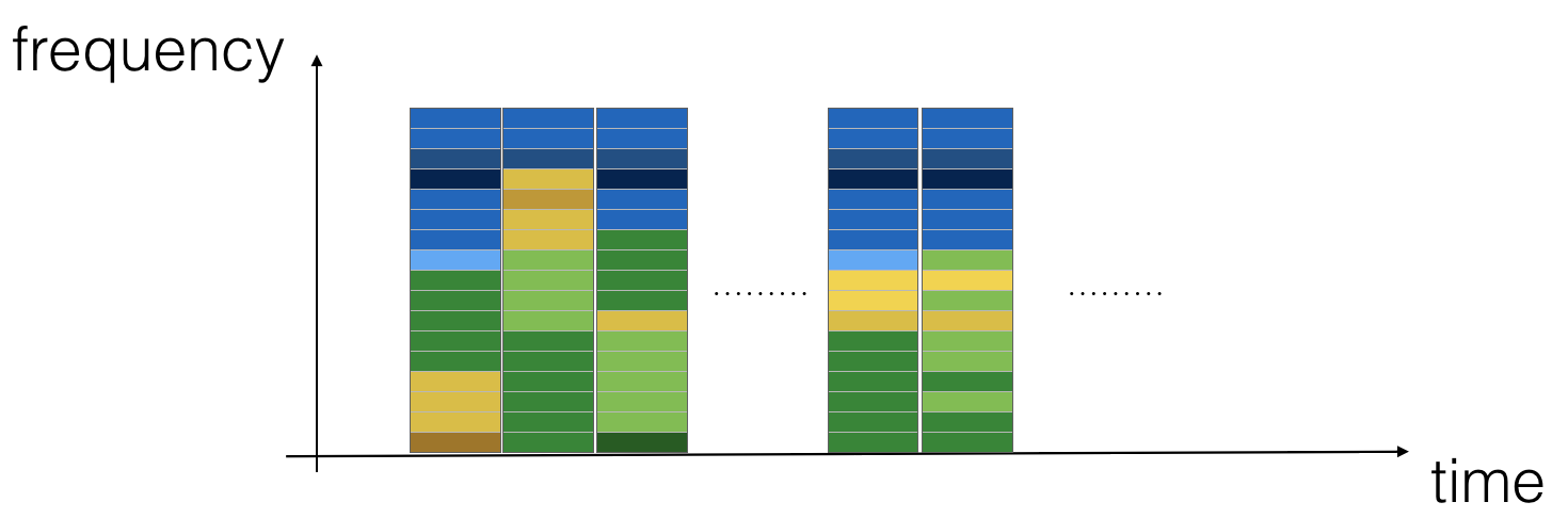
音频录制的频谱图,其中颜色显示不同时间点音频中不同频率(大声)的存在程度。 绿色方块表示某个频率在音频片段中更活跃或更多(更响亮); 蓝色方块表示较不活跃的频率。
输出频谱图的尺寸取决于频谱图软件的pydub模块使用它来合成音频超参数和输入的长度。 在这款笔记本中,我们将使用10秒的音频剪辑作为我们培训示例的“标准长度”。 频谱图的时间步长为5511.稍后您将看到频谱图将是进入网络的输入x,因此Tx = 5511。
输出频谱图的尺寸取决于频谱图软件的超参数和输入的长度。 这里,我们将使用10秒音频剪辑作为我们培训示例的“标准长度”。 频谱图的时间步长为5511.稍后您将看到频谱图将是输入网络的 $ x $ ,因此 $ T_x = 5511 $。
_, data = wavfile.read("audio_examples/example_train.wav")
print("Time steps in audio recording before spectrogram", data[:,0].shape)
print("Time steps in input after spectrogram(频谱)", x.shape)
Time steps in audio recording before spectrogram (441000,)
Time steps in input after spectrogram(频谱) (101, 5511)
现在你可以定义:
Tx = 5511 # 从频谱图输入到模型的时间步数
#The number of time steps input to the model from the spectrogram
n_freq = 101 # 在频谱图的每个时间步输入模型的频率数
#Number of frequencies input to the model at each time step of the spectrogram
请注意,即使我们的默认训练示例长度为10秒,也可以将10秒的时间离散化为不同的值。你已经看过441000(原始音频)和5511(频谱图 spectrogram)。在前一种情况下,每一步代表\(10/441000 \approx 0.000023\)秒。在第二种情况下,每一步代表\(10/5511 \approx 0.0018\) 秒。
对于10秒的音频,您将在此作业中看到的键值为:
- \(10000\) (由
pydub模块用于合成音频) - \(1375 = T_y\) (将构建的GRU输出中的步)
请注意,这些表示中的每一个 each of these representations 都恰好对应于10秒的时间。只是他们在不同程度上将它们离散化。所有这些都是超参数并且可以更改(除了441000,这是麦克风的功能)。我们选择了语音系统标准范围内的值。
考虑上面的$ T_y = 1375 $数字。这意味着对于模型的输出,我们将10s离散化为1375个时间间隔 (each one of length \(10/1375 \approx 0.0072\)s),并尝试预测每个时间间隔是否有人最近说完“activate”。 “
还要考虑上面的10000号码。这相当于将10秒剪辑离散化为10/10000 = 0.001秒的间隔itervals。 0.001秒也称为1 millisecond 毫秒,或1ms。因此,当我们说我们按照1ms间隔进行离散化时,这意味着我们使用了10,000步。
Ty = 1375 # The number of time steps in the output of our model
1.3 - 生成单个训练示例
由于语音数据难以获取和标记,因此您将使用 activates,negatives和backgrounds的音频剪辑合成训练数据。 录制大量10秒音频片段并且其中有随机“activates”是很慢的。 相反,我们更容易记录大量的正面和负面词,并分别记录背景噪音(或从免费在线资源下载背景噪音)。
要综合单个训练示例,您将:
- 选择一个随机的10秒背景音频剪辑
- 随机插入0-4个"activate"到这个10秒剪辑
- 随机插入0-2个 negative words 到这个10秒剪辑
因为您已将“activate”一词合成到背景剪辑中,所以明确知道在10秒剪辑中“activate”出现的时间。 稍后您会看到,这样也可以更容易地生成label \(y^{\langle t \rangle}\)
您将使用pydub包来合成音频。 Pydub将原始音频文件转换为Pydub数据结构列表 lists of Pydub data structures(这里了解详细信息并不重要)。 Pydub使用1ms作为离散化间隔discretization interval(1ms是1毫秒= 1/1000秒),这就是为什么10sec剪辑总是用10,000步表示的原因。
# Load audio segments using pydub
activates, negatives, backgrounds = load_raw_audio()

print("background len: " + str(len(backgrounds[0])))    # Should be 10,000, since it is a 10 sec clip
print("activate[0] len: " + str(len(activates[0])))     # Maybe around 1000, since an "activate" audio clip is usually around 1 sec (but varies a lot)
print("activate[1] len: " + str(len(activates[1])))     # Different "activate" clips can have different lengths
background len: 10000
activate[0] len: 721
activate[1] len: 731
在背景上合成 positive/negative 单词:
给定10秒背景剪辑和短音频剪辑(正面或负面单词),您需要能够将单词的短音频剪辑“添加”或“插入”到背景音频上。 为了确保插入到背景中的音频片段不重叠,您将跟踪先前插入的音频片段的时间。 您将在背景上插入多个positive/negative单词的剪辑,并且您不希望在某个与您之前添加的另一个剪辑重叠的地方插入“activate”或随机字。
为了清楚起见,当您在咖啡馆噪音的10秒剪辑中插入1秒“activate”时,您最终得到一个10秒的剪辑,听起来像某人在咖啡馆中“激活”,“activate”叠加在背景咖啡厅噪音上。 你没有不会得到一个11秒的剪辑。 稍后您将看到pydub如何完成它。
在叠加的同时创建标签:::
回想一下,标签 \(y^{\langle t \rangle}\) 表示某人是否刚刚说完“激活”。 给定背景剪辑,我们可以为所有\(t\)初始化\(y^{\langle t \rangle}=0\) ,因为剪辑不包含任何“activates”。
当您插入或覆盖“activate”剪辑时,您还将更新\(y^{\langle t \rangle}\),以便输出的50 steps具有target label 1. 您将训练GRU以检测何时有人完成说“activate”。 例如,假设合成的“activate”剪辑在10秒音频中的5秒标记处结束---正好在剪辑的一半处。 回想一下$ T_y = 1375 $,所以时间步 $687 = $ int(1375*0.5) 对应于5秒进入音频的那一刻。 所以,你将设置\(y^{\langle 688 \rangle} = 1\)。 此外,如果GRU在说完的短时间内检测到“activate”,你会非常满意,因此我们实际上将标签\(y^{\langle t \rangle}\)的50个连续值设置为1.具体来说, 我们有\(y^{\langle 688 \rangle} = y^{\langle 689 \rangle} = \cdots = y^{\langle 737 \rangle} = 1\)。
这是合成训练数据的另一个原因:如上所述生成这些标签\(y^{\langle t \rangle}\)相对简单。 相比之下,如果您在麦克风上录制了10秒的音频,那么一个人收听它并在"activate" 完成后手动标记是非常耗时的。
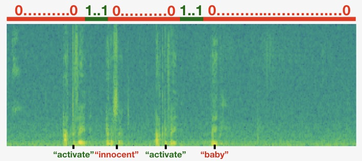
这是一个图形说明标签 \(y^{\langle t \rangle}\),我们插入“activate”,“innocent”,activate“,”baby“ 的剪辑。 注意,正面标签”1“是只关联 positive words。
要实现训练集合成过程,您将使用以下辅助函数。 所有这些功能都将使用1ms的离散化间隔,因此10秒的音频可以离散化为10,000步。
1.get_random_time_segment(segment_ms)在我们的背景音频中获得一个随机时间段
2.is_overlapping(segment_time,existing_segments)检查时间段是否与现有段重叠
3.insert_audio_clip(background,audio_clip,existing_times)使用get_random_time_segment和is_overlapping在我们的背景音频中随机插入音频片段。
4.insert_ones(y,segment_end_ms)在“activate”一词之后将1插入到我们的标签向量y中
函数get_random_time_segment(segment_ms)返回一个随机时间段,我们可以在其上插入持续时间为segment_ms的音频剪辑。 仔细阅读代码,确保您了解它的作用。
def get_random_time_segment(segment_ms):
    """
    Gets a random time segment of duration segment_ms in a 10,000 ms audio clip.

    Arguments:
    segment_ms -- the duration of the audio clip in ms ("ms" stands for "milliseconds")

    Returns:
    segment_time -- a tuple of (segment_start, segment_end) in ms
    """
    #10秒的音频10000 steps, 随机选择一个初始点
    segment_start = np.random.randint(low=0, high=10000-segment_ms)   # Make sure segment doesn't run past the 10sec background
    segment_end = segment_start + segment_ms - 1

    return (segment_start, segment_end)
接下来,假设您已在段(1000,1800)和(3400,4500)处插入音频剪辑。 即,第一段从步骤1000开始,并在步骤1800结束。现在,如果我们正在考虑在(3000,3600)处插入新的音频片段,这是否与先前插入的片段之一重叠? 在这种情况下,(3000,3600)和(3400,4500)重叠,所以我们应该决定不在这里插入一个剪辑。
出于该功能的目的,定义(100,200)和(200,250)是重叠的,因为它们在时间步长200处重叠。但是,(100,199)和(200,250)是不重叠的。
练习:实现is_overlapping(segment_time,existing_segments)来检查新的时间段是否与任何先前的段重叠。 您需要执行两个步骤:
1.创建一个“False”标志,如果发现存在重叠,稍后将设置为“True”。
2.遍历previous_segments的开始和结束时间。 将这些时间与段的开始和结束时间进行比较。 如果存在重叠,请将(1)中定义的标志设置为True。 您可以使用:
for ....:
        if ... <= ... and ... >= ...:
            ...
提示:如果段 segment 在前一段结束之前开始,并且段在前一段开始之后结束 是重叠。
Hint: There is overlap if the starts before the previous segment ends, and the segment ends after the previous segment starts.
# GRADED FUNCTION: is_overlapping

def is_overlapping(segment_time, previous_segments):
    """
    Checks if the time of a segment overlaps with the times of existing segments.

    Arguments:
    segment_time -- a tuple of (segment_start, segment_end) for the new segment
    previous_segments -- a list of tuples of (segment_start, segment_end) for the existing segments
    #当前存在的所有插入的时间段集合 (segment_start, segment_end)
    Returns:
    True if the time segment overlaps with any of the existing segments, False otherwise
    """

    segment_start, segment_end = segment_time

    ### START CODE HERE ### (≈ 4 line)
    # Step 1: Initialize overlap as a "False" flag. (≈ 1 line)
    overlap = False

    # Step 2: loop over the previous_segments start and end times.
    # Compare start/end times and set the flag to True if there is an overlap (≈ 3 lines)
    for previous_start, previous_end in previous_segments:
        if segment_start >= previous_start and segment_start <= previous_end:
            overlap = True
    ### END CODE HERE ###

    return overlap
overlap1 = is_overlapping((950, 1430), [(2000, 2550), (260, 949)])
overlap2 = is_overlapping((2305, 2950), [(824, 1532), (1900, 2305), (3424, 3656)])
print("Overlap 1 = ", overlap1)
print("Overlap 2 = ", overlap2)
Overlap 1 =  False
Overlap 2 =  True
Expected Output:
| **Overlap 1** | False |
| **Overlap 2** | True |
现在,让我们使用以前的辅助函数在随机时间将新的音频剪辑插入到10sec背景上,但确保任何新插入的片段不会与之前的片段重叠。
练习:实现insert_audio_clip()将音频片段叠加到背景10秒片段上。 您需要执行4个步骤:
1.以ms为单位获取正确持续时间的随机时间段。
2.确保时间段不与之前的任何时间段重叠。 如果它重叠,则返回步骤1并选择一个新的时间段。
3.将新时间段添加到现有时间段列表中,以便跟踪您插入的所有时间段。
4.使用pydub在背景上叠加音频片段。 我们已经为您实现了这一点。
# GRADED FUNCTION: insert_audio_clip

def insert_audio_clip(background, audio_clip, previous_segments):
    """
    Insert a new audio segment over the background noise at a random time step, ensuring that the
    audio segment does not overlap with existing segments.

    Arguments:
    background -- a 10 second background audio recording.
    audio_clip -- the audio clip to be inserted/overlaid.
    previous_segments -- times where audio segments have already been placed

    Returns:
    new_background -- the updated background audio
    """

    # Get the duration of the audio clip in ms
    segment_ms = len(audio_clip) #需要插入的音频的长度(ms)

    ### START CODE HERE ###
    # Step 1: Use one of the helper functions to pick a random time segment onto which to insert
    # the new audio clip. (≈ 1 line)
    segment_time = get_random_time_segment(segment_ms)

    # Step 2: Check if the new segment_time overlaps with one of the previous_segments. If so, keep
    # picking new segment_time at random until it doesn't overlap. (≈ 2 lines)
    while is_overlapping(segment_time, previous_segments):
        segment_time = get_random_time_segment(segment_ms)

    # Step 3: Add the new segment_time to the list of previous_segments (≈ 1 line)
    previous_segments.append(segment_time)
    ### END CODE HERE ###

    # Step 4: Superpose audio segment and background 合成新的声音
    new_background = background.overlay(audio_clip, position = segment_time[0])

    return new_background, segment_time
np.random.seed(5)
audio_clip, segment_time = insert_audio_clip(backgrounds[0], activates[0], [(3790, 4400)])
audio_clip.export("insert_test.wav", format="wav")
print("Segment Time: ", segment_time)
IPython.display.Audio("insert_test.wav")
Expected Output
| **Segment Time** | (2254, 3169) |
# Expected audio
IPython.display.Audio("audio_examples/insert_reference.wav")
最后,使用代码更新标签\(y^{\langle t \rangle}\),假设您刚刚插入了“activate”。 在下面的代码中,y是一个(1,1375)维向量,因为$ T_y = 1375 $。
如果“activate”在时间步\(t\)结束,则设置\(y^{\langle t+1 \rangle} = 1\)以及后面最多49个附加连续值为1。 但是,请确保不要运行到数组的末尾并尝试更新y [0] [1375],因为有效索引是y [0] [0]到y [0] [ 1374] 因为$ T_y = 1375 $。 因此,如果“激活”在步骤1370结束,则仅得到 y[0][1371] = y[0][1372] = y[0][1373] = y[0][1374] = 1
练习:实现insert_ones()。 你可以使用for循环。(如果你会使用python切片操作,也可以使用切片来对其进行矢量化。)如果一个段以segment_end_ms结尾(使用10000 step discretization),则将其转换为输出的索引 \(y\) (使用$ 1375 $ step discretization),我们将使用以下公式:
segment_end_y = int(segment_end_ms * Ty / 10000.0)
# GRADED FUNCTION: insert_ones

def insert_ones(y, segment_end_ms):
    """
    Update the label vector y. The labels of the 50 output steps strictly after the end of the segment
    should be set to 1. By strictly we mean that the label of segment_end_y should be 0 while, the
    50 followinf labels should be ones.


    Arguments:
    y -- numpy array of shape (1, Ty), the labels of the training example
    segment_end_ms -- the end time of the segment in ms

    Returns:
    y -- updated labels
    """

    # duration of the background (in terms of spectrogram time-steps)
    segment_end_y = int(segment_end_ms * Ty / 10000.0)
    # segment_end_y / Ty = segment_end_ms (activate结束step) / 10000 (总的step)

    # Add 1 to the correct index in the background label (y)
    ### START CODE HERE ### (≈ 3 lines)
    for i in range(segment_end_y + 1, segment_end_y + 51):
        if i < Ty:
            y[0, i] = 1
    ### END CODE HERE ###

    return y
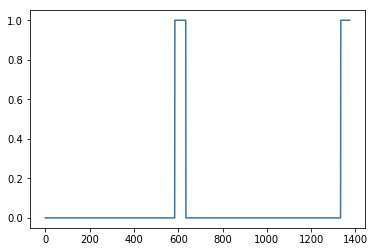
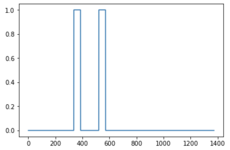
arr1 = insert_ones(np.zeros((1, Ty)), 9700)
plt.plot(insert_ones(arr1, 4251)[0,:])
print("sanity checks:", arr1[0][1333], arr1[0][634], arr1[0][635])
sanity checks: 0.0 1.0 0.0
最后,您可以使用insert_audio_clip和insert_ones来创建一个新的训练示例。
练习:实现create_training_example()。 您需要执行以下步骤:
1.将标签向量$ y $初始化为numpy数组,shape \((1,T_y)\)。
2.将 existing segments的集合初始化为空列表。
3.随机选择0到4个“activate”音频剪辑,然后将它们插入10秒剪辑。 还要在标签向量$ y $中的正确位置插入标签。
4.随机选择0到2个负音频剪辑,并将它们插入10秒剪辑中。
# GRADED FUNCTION: create_training_example

def create_training_example(background, activates, negatives):
    """
    Creates a training example with a given background, activates, and negatives.

    Arguments:
    background -- a 10 second background audio recording
    activates -- a list of audio segments of the word "activate"
    negatives -- a list of audio segments of random words that are not "activate"

    Returns:
    x -- the spectrogram of the training example
    y -- the label at each time step of the spectrogram
    """

    # Set the random seed
    np.random.seed(18)

    # Make background quieter
    background = background - 20

    ### START CODE HERE ###
    # Step 1: Initialize y (label vector) of zeros (≈ 1 line)
    y = np.zeros((1, Ty))

    # Step 2: Initialize segment times as empty list (≈ 1 line)
    previous_segments = []
    ### END CODE HERE ###

    # Select 0-4 random "activate" audio clips from the entire list of "activates" recordings
    number_of_activates = np.random.randint(0, 5)
    #print(number_of_activates)
    random_indices = np.random.randint(len(activates), size=number_of_activates)
    random_activates = [activates[i] for i in random_indices]

    ### START CODE HERE ### (≈ 3 lines)
    # Step 3: Loop over randomly selected "activate" clips and insert in background
    for random_activate in random_activates:
        # Insert the audio clip on the background
        background, segment_time = insert_audio_clip(background, random_activate, previous_segments)
        # Retrieve segment_start and segment_end from segment_time
        segment_start, segment_end = segment_time
        # Insert labels in "y"
        y = insert_ones(y, segment_end)
    ### END CODE HERE ###

    # Select 0-2 random negatives audio recordings from the entire list of "negatives" recordings
    number_of_negatives = np.random.randint(0, 3)
    random_indices = np.random.randint(len(negatives), size=number_of_negatives)
    random_negatives = [negatives[i] for i in random_indices]

    ### START CODE HERE ### (≈ 2 lines)
    # Step 4: Loop over randomly selected negative clips and insert in background
    for random_negative in random_negatives:
        # Insert the audio clip on the background
        background, _ = insert_audio_clip(background, random_negative, previous_segments)
    ### END CODE HERE ###

    # Standardize the volume of the audio clip
    background = match_target_amplitude(background, -20.0)

    # Export new training example
    file_handle = background.export("train" + ".wav", format="wav")
    print("File (train.wav) was saved in your directory.")

    # Get and plot spectrogram of the new recording (background with superposition of positive and negatives)
    x = graph_spectrogram("train.wav")

    return x, y
x, y = create_training_example(backgrounds[0], activates, negatives)
File (train.wav) was saved in your directory.


D:\software\Anaconda3\envs\tensorflow\lib\site-packages\matplotlib\axes\_axes.py:7674: RuntimeWarning: divide by zero encountered in log10
  Z = 10. * np.log10(spec)
现在,您可以聆听您创建的训练示例,并将其与上面生成的频谱图进行比较。
IPython.display.Audio("train.wav")
Expected Output
IPython.display.Audio("audio_examples/train_reference.wav")
最后,您可以绘制生成的训练示例的关联标签。
plt.plot(y[0])
Expected Output
1.4 - 完整的训练集
您现在已经实现了生成单个训练示例所需的代码。 我们使用此过程生成一个大型训练集。 为了节省时间,我们已经生成了一组训练样本。
# Load preprocessed training examples
X = np.load("./XY_train/X.npy")
Y = np.load("./XY_train/Y.npy")
1.5 - Development set
为了测试我们的模型,我们记录了一个包含25个示例的development set。 虽然我们的训练数据是合成的,但我们希望使用与实际输入相同的分布来创建development set。 因此,我们录制了25个10秒钟的人们说“activate”和其他随机单词的音频剪辑,并用手标记。 这遵循课程3中描述的原则,即我们应该将dev set设置为尽可能与测试集分布相似; 这就是我们的 dev set使用真实而非合成音频的原因。
# Load preprocessed dev set examples
X_dev = np.load("./XY_dev/X_dev.npy")
Y_dev = np.load("./XY_dev/Y_dev.npy")
2 - 模型
现在您已经构建了一个数据集,让我们编写并训练一个触发词检测模型!
该模型将使用1-D卷积层,GRU层和密集层。 让我们加载允许您在Keras中使用这些图层的包。 这可能需要一分钟才能加载。
from keras.callbacks import ModelCheckpoint
from keras.models import Model, load_model, Sequential
from keras.layers import Dense, Activation, Dropout, Input, Masking, TimeDistributed, LSTM, Conv1D
from keras.layers import GRU, Bidirectional, BatchNormalization, Reshape
from keras.optimizers import Adam
D:\software\Anaconda3\envs\tensorflow\lib\importlib\_bootstrap.py:222: RuntimeWarning: numpy.dtype size changed, may indicate binary incompatibility. Expected 88 from C header, got 96 from PyObject
  return f(*args, **kwds)
Using TensorFlow backend.
2.1 - 建立模型
这是我们将使用的架构。 花一些时间来查看模型,看看它是否有意义。
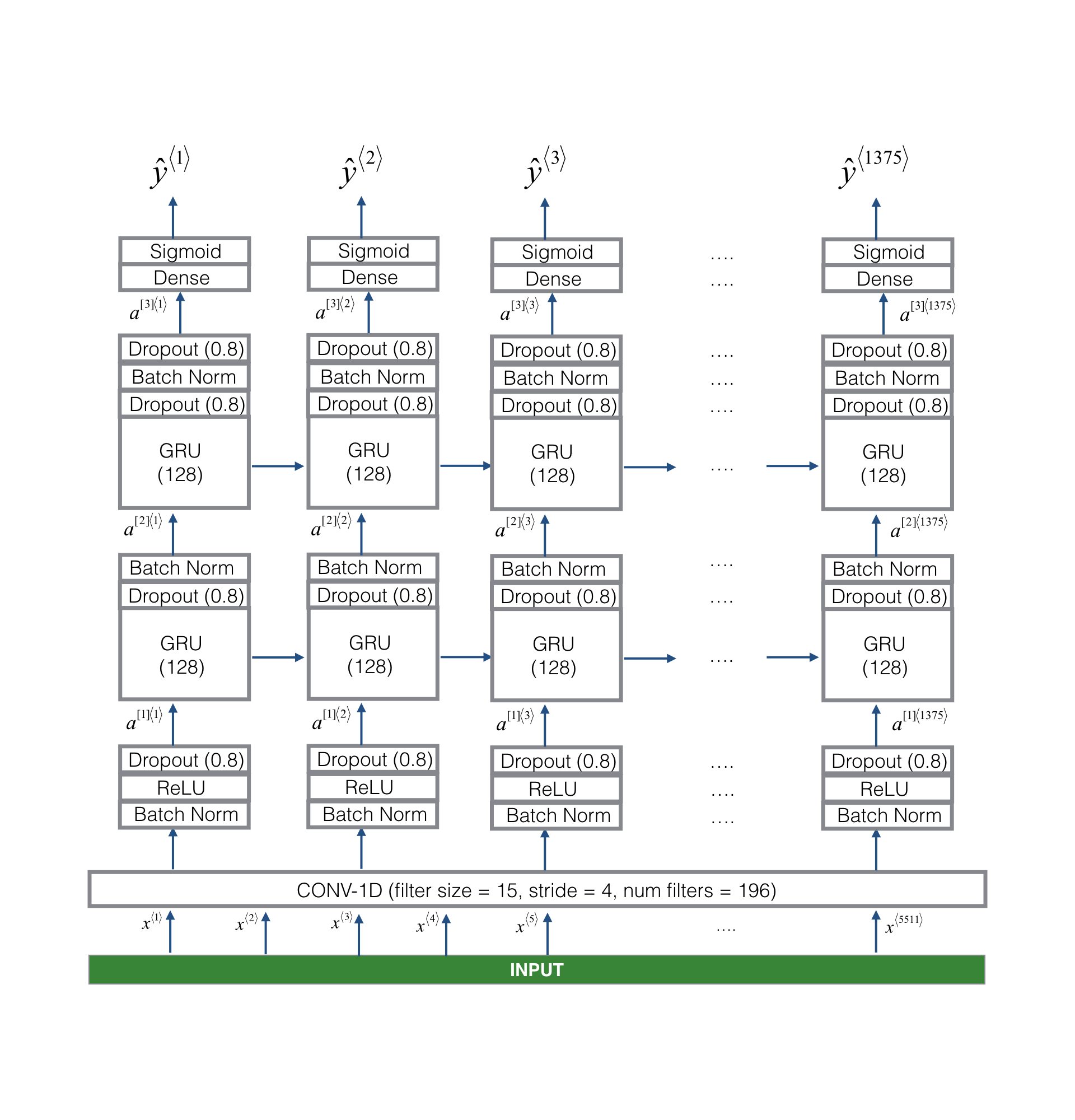
该模型的一个关键步骤是1D卷积步骤(靠近图3的底部)。它输入5511步的频谱,并输出一个1375步输出,然后由多个层进一步处理,以获得最终的$ T_y = 1375 $步输出。该层的作用类似于您在课程4中看到的2D卷积层(这里是1D),提取低级特征(low-level features),然后可能生成较小维度的输出。
在计算上,1-D转换层(conv layer)也有助于加速模型,因为现在GRU只需要处理1375个时间步而不是5511个时间步。两个GRU层从左到右读取输入序列,然后最终使用dense+sigmoid层来预测\(y^{\langle t \rangle}\)。因为\(y\)是二进制值(0或1),我们在最后一层使用sigmoid输出来估计输出为1的概率,对应于用户刚刚说“activate”。
请注意,我们使用单向RNN而不是双向RNN。这对于触发字检测非常重要,因为我们希望能够在说出触发字后立即检测到触发字(detect the trigger word almost immediately after it is said)。如果我们使用双向RNN,我们必须等待整个10秒的音频被记录,然后才能判断音频片段的第一秒是否有“激活”。
实现模型可以分四步完成:
步骤1:CONV层。使用Conv1D()来实现这一点,使用196个过滤器,
过滤器大小为15(kernel_size = 15),步幅stride为4. [See documentation.]
步骤2:第一个GRU层。要生成GRU图层,请使用:
X = GRU(units = 128, return_sequences = True)(X)
设置return_sequences = True可确保将所有GRU的隐藏状态喂给下一层。请记住使用Dropout和BatchNorm层。
步骤3:第二个GRU层。这类似于以前的GRU层(记得使用return_sequences = True),但有一个额外的dropout层。
步骤4:创建时间分布time-distributed 的 dense layer,如下所示:
X = TimeDistributed(Dense(1, activation = "sigmoid"))(X)
这将创建一个密集的层,后跟一个sigmoid,因此用于密集层的参数对于每个时间步都是相同的。[See documentation.]
练习:实现model(),体系结构如图3所示。
# GRADED FUNCTION: model

def model(input_shape):
    """
    Function creating the model's graph in Keras.

    Argument:
    input_shape -- shape of the model's input data (using Keras conventions)

    Returns:
    model -- Keras model instance
    """

    X_input = Input(shape = input_shape)

    ### START CODE HERE ###

    # Step 1: CONV layer (≈4 lines)
    X = Conv1D(196, 15, strides=4)(X_input)     # CONV1D
    X = BatchNormalization()(X)                 # Batch normalization
    X = Activation('relu')(X)                   # ReLu activation
    X = Dropout(0.8)(X)                         # dropout (use 0.8)

    # Step 2: First GRU Layer (≈4 lines)
    X = GRU(128, return_sequences=True)(X)      # GRU (use 128 units and return the sequences)
    X = Dropout(0.8)(X)                         # dropout (use 0.8)
    X = BatchNormalization()(X)                 # Batch normalization

    # Step 3: Second GRU Layer (≈4 lines)
    X = GRU(128, return_sequences=True)(X)   # GRU (use 128 units and return the sequences)
    X = Dropout(0.8)(X)                      # dropout (use 0.8)
    X = BatchNormalization()(X)              # Batch normalization
    X = Dropout(0.8)(X)                      # dropout (use 0.8)

    # Step 4: Time-distributed dense layer (≈1 line)
    X = TimeDistributed(Dense(1, activation = "sigmoid"))(X) # time distributed  (sigmoid)

    ### END CODE HERE ###

    model = Model(inputs = X_input, outputs = X)

    return model
model = model(input_shape = (Tx, n_freq))
让我们打印模型摘要以跟踪形状。
model.summary()
_________________________________________________________________
Layer (type)                 Output Shape              Param #
=================================================================
input_2 (InputLayer)         (None, 5511, 101)         0
_________________________________________________________________
conv1d_2 (Conv1D)            (None, 1375, 196)         297136
_________________________________________________________________
batch_normalization_4 (Batch (None, 1375, 196)         784
_________________________________________________________________
activation_2 (Activation)    (None, 1375, 196)         0
_________________________________________________________________
dropout_5 (Dropout)          (None, 1375, 196)         0
_________________________________________________________________
gru_3 (GRU)                  (None, 1375, 128)         124800
_________________________________________________________________
dropout_6 (Dropout)          (None, 1375, 128)         0
_________________________________________________________________
batch_normalization_5 (Batch (None, 1375, 128)         512
_________________________________________________________________
gru_4 (GRU)                  (None, 1375, 128)         98688
_________________________________________________________________
dropout_7 (Dropout)          (None, 1375, 128)         0
_________________________________________________________________
batch_normalization_6 (Batch (None, 1375, 128)         512
_________________________________________________________________
dropout_8 (Dropout)          (None, 1375, 128)         0
_________________________________________________________________
time_distributed_2 (TimeDist (None, 1375, 1)           129
=================================================================
Total params: 522,561
Trainable params: 521,657
Non-trainable params: 904
_________________________________________________________________
Expected Output:
| **Total params** | 522,561 |
| **Trainable params** | 521,657 |
| **Non-trainable params** | 904 |
网络的输出是形状(None, 1375, 1) ,而输入是(None, 5511, 101)。 Conv1D将频谱的步数(steps)从5511减少到1375。
2.2 - Fit the model
触发字检测需要很长时间才能进行训练。 为了节省时间,我们已经使用您在上面构建的架构在GPU上训练了大约3个小时的模型,以及大约4000个示例的大型训练集。 让我们加载模型。
model = load_model('./models/tr_model.h5')
D:\software\Anaconda3\envs\tensorflow\lib\site-packages\keras\engine\saving.py:327: UserWarning: Error in loading the saved optimizer state. As a result, your model is starting with a freshly initialized optimizer.
  warnings.warn('Error in loading the saved optimizer '
您可以使用Adam优化器和二进制交叉熵损失来进一步训练模型(train the model further),如下所示。 这将很快运行,因为我们只训练一个epoch,并且训练集包含26个样本。
opt = Adam(lr=0.0001, beta_1=0.9, beta_2=0.999, decay=0.01)
model.compile(loss='binary_crossentropy', optimizer=opt, metrics=["accuracy"])
model.fit(X, Y, batch_size = 5, epochs=1)
Epoch 1/1
26/26 [==============================] - 7s 286ms/step - loss: 0.0582 - acc: 0.9815


<keras.callbacks.History at 0x44923128>
2.3 - 测试模型
最后,让我们看看您的模型在dev set上的表现。
loss, acc = model.evaluate(X_dev, Y_dev)
print("Dev set accuracy = ", acc)
25/25 [==============================] - 1s 52ms/step
Dev set accuracy =  0.9406254291534424
这看起来很不错! 然而,准确性对于这项任务来说并不是一个很好的指标,因为标签严重偏向0,因此只输出0的神经网络将获得略高于90%的准确度。 我们可以定义更多有用的指标,例如F1得分或精确/召回。 但是,让我们不要在这里困扰这些,而只是凭经验看到模型是如何做的。
3 - 做出预测
现在您已经为触发词检测构建了一个工作模型,让我们用它来进行预测。 此代码段通过网络运行音频(保存在wav文件中)。
可以使用您的模型对新的音频剪辑进行预测。您首先需要计算输入音频剪辑的预测。
练习:实现predict_activates()。 您需要执行以下操作:
1.计算音频文件的频谱图(spectrogram)
2.使用np.swap和np.expand_dims将输入重新整形为大小(1,Tx,n_freqs)
3.在模型上使用向前传播来计算每个输出步骤的预测
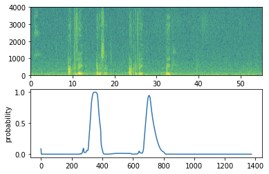
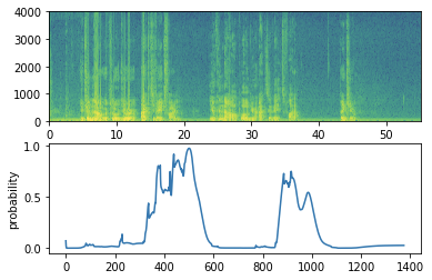
def detect_triggerword(filename):
    plt.subplot(2, 1, 1)

    x = graph_spectrogram(filename)
    # the spectogram outputs (freqs, Tx) and we want (Tx, freqs) to input into the model
    x  = x.swapaxes(0,1)
    x = np.expand_dims(x, axis=0)
    predictions = model.predict(x)

    plt.subplot(2, 1, 2)
    plt.plot(predictions[0,:,0])
    plt.ylabel('probability')
    plt.show()
    return predictions
一旦您估计了在每个输出步骤检测到“activate”一词的概率,您就可以在概率超过某个阈值时触发“鸣响”声音。此外,\(y^{\langle t \rangle}\)可能在接近“activate”之后连续的多个值接近1,但我们只想响一次。因此,我们将每75个输出步骤最多产生一次铃声(产生一次后,下75个时间步内不产生)。这将有助于防止我们为单个“activate”实例插入两个钟声。 (这与计算机视觉中的非最大抑制 non-max suppression 类似。)
练习:实现chime_on_activate()。您需要执行以下操作:
1.在每个输出步骤循环预测概率
2.当预测值大于阈值且超过75个连续时间步长时,在原始音频片段上插入“chime”声音
使用下面代码将1,375步离散化转换为10,000步离散化,并使用pydub插入“chime”:
audio_clip = audio_clip.overlay(chime,position =((i / Ty)* audio.duration_seconds)* 1000)
chime_file = "audio_examples/chime.wav"
def chime_on_activate(filename, predictions, threshold):
    audio_clip = AudioSegment.from_wav(filename)
    chime = AudioSegment.from_wav(chime_file)
    Ty = predictions.shape[1]
    # Step 1: Initialize the number of consecutive output steps to 0
    consecutive_timesteps = 0
    # Step 2: Loop over the output steps in the y
    for i in range(Ty):
        # Step 3: Increment consecutive output steps
        consecutive_timesteps += 1
        # Step 4: If prediction is higher than the threshold and more than 75 consecutive output steps have passed
        if predictions[0,i,0] > threshold and consecutive_timesteps > 75:
            # Step 5: Superpose audio and background using pydub
            audio_clip = audio_clip.overlay(chime, position = ((i / Ty) * audio_clip.duration_seconds)*1000)
            # Step 6: Reset consecutive output steps to 0
            consecutive_timesteps = 0

    audio_clip.export("chime_output.wav", format='wav')
3.3 - Test on dev examples
让我们探索一下我们的模型如何在development set中的两个看不见的音频剪辑上执行。 让我们先听两个dev set的剪辑。
IPython.display.Audio("./raw_data/dev/1.wav")
IPython.display.Audio("./raw_data/dev/2.wav")
现在让我们在这些音频片段上运行模型,看看它是否在“activate”后添加了一个铃声!
filename = "./raw_data/dev/1.wav"
prediction = detect_triggerword(filename)
chime_on_activate(filename, prediction, 0.5)
IPython.display.Audio("./chime_output.wav")

filename  = "./raw_data/dev/2.wav"
prediction = detect_triggerword(filename)
chime_on_activate(filename, prediction, 0.5)
IPython.display.Audio("./chime_output.wav")
Congratulations
这是你应该记住的:
- 数据合成是为语音问题创建大型训练集的有效方法,特别是触发单词检测。
- 在将音频数据传递到RNN,GRU或LSTM之前,使用频谱图和可选的1D conv layer是常见的预处理步骤。
- 端到端 end-to-end 深度学习方法可用于构建非常有效的触发字检测系统。
恭喜你完成了最终的任务!
感谢您坚持到最后,并为您学习深度学习所付出的辛勤劳动。 我们希望您喜欢这门课程!
4 - 试试你自己样本! (OPTIONAL/UNGRADED)
您可以在自己的音频剪辑上试用您的模型!
录制你说“activate”和其他随机单词的10秒音频片段,并将其作为“myaudio.wav”上传到Coursera集线器。 请务必将音频上传为wav文件。 如果您的音频以不同的格式(例如mp3)录制,则可以在线找到将其转换为wav的免费软件。 如果您的录音时间不是10秒,则下面的代码将根据需要修剪或填充它以使其达到10秒。
# Preprocess the audio to the correct format
def preprocess_audio(filename):
    # Trim or pad audio segment to 10000ms
    padding = AudioSegment.silent(duration=10000)
    segment = AudioSegment.from_wav(filename)[:10000]
    segment = padding.overlay(segment)
    # Set frame rate to 44100
    segment = segment.set_frame_rate(44100)
    # Export as wav
    segment.export(filename, format='wav')
Once you've uploaded your audio file to Coursera, put the path to your file in the variable below.
your_filename = "audio_examples/my_audio.wav"
preprocess_audio(your_filename)
IPython.display.Audio(your_filename) # listen to the audio you uploaded
最后,使用模型预测何时在10秒音频片段中激活,并触发铃声。 如果没有正确添加蜂鸣声,请尝试调整chime_threshold。
chime_threshold = 0.5
prediction = detect_triggerword(your_filename)
chime_on_activate(your_filename, prediction, chime_threshold)
IPython.display.Audio("./chime_output.wav")

 浙公网安备 33010602011771号