人工智能实战_第五次作业_廖盈嘉
第5次作业:逻辑与门和逻辑或门
| 项目 | 内容 |
|---|---|
| 这个作业属于哪个课程 | |
| 这个作业的要求在哪里 | |
| 我在这个课程的目标是 | 学会、理解和应用神经网络知识来完成一个app |
| 这个作业在哪个具体方面帮助我实现目标 | 学会使用sigmoid激活函数和二分类交叉熵函损失数 |
| 作业正文 | |
| 参考文献 |
一、作业要求
- 训练逻辑与门和逻辑或门结果及代码形成博客
二、样本和特征
1. 逻辑与门的样本和特征
| Example | 1 |
2 |
3 |
4 |
|---|---|---|---|---|
| X1 | 0 |
0 |
1 |
1 |
| X2 | 0 |
1 |
0 |
1 |
| Y | 0 |
0 |
0 |
1 |
2. 逻辑或门的样本和特征
| Example | 1 |
2 |
3 |
4 |
|---|---|---|---|---|
| X1 | 0 |
0 |
1 |
1 |
| X2 | 0 |
1 |
0 |
1 |
| Y | 0 |
1 |
1 |
1 |
三、引用公式
1. 激活函数,$A = sigmoid(Z) = \frac{1}{1+e^-Z}$
2. 二分类交叉熵函损失数Cross Entropy, \(J = -[YlnA + (1-Y)ln(1-A)]\)
3. 直线方程: $x_2 = \frac{w_1}{w_2}x_1\ - \frac{b}{w_2}$
四、代码实现
整体代码
import numpy as np
import matplotlib.pyplot as plt

def ReadData(logic):
    if logic == "OR":
        X = np.array([0,0,1,1,0,1,0,1]).reshape(2,4)
        Y = np.array([0,1,1,1]).reshape(1,4)
    elif logic == "AND":
        X = np.array([0,0,1,1,0,1,0,1]).reshape(2,4)
        Y = np.array([0,0,0,1]).reshape(1,4)
    return X,Y

def sigmoid(x):
    # sigmoid function (activation function)
    S = 1/(1+np.exp(-x))
    return S

def ForwardCalculation(w,b,x):
    z = np.dot(w, x) + b
    # After calculating Z, Z needs to be passed into sigmoid activation function
    A = sigmoid(z)
    return A

def BackPropagation(x,y,A,num_example):
    dZ = A - y
    dB = dZ.sum(axis=1, keepdims=True)/num_example
    dW = np.dot(dZ, x.T)/num_example
    return dW, dB

def UpdateWeights(w, b, dW, dB, eta):
    w = w - eta*dW
    b = b - eta*dB
    return w,b

def CheckLoss(w, b, X, Y, num_example):
    m = num_example
    A = ForwardCalculation(w,b,X)

    # Cross Entropy Equation for loss: J = -(1/m)sum{[YlnA + (1-Y)ln(1-A)]}
    n1 = 1 - Y
    n2 = np.log(1-A)
    n3 = np.log(A)
    n4 = np.multiply(n1,n2)
    n5 = np.multiply(Y,n3)

    LOSS = np.sum(-(n4 + n5))
    loss = LOSS/m
    return loss

def ShowResult(w,b,X,Y,num_example,logic):
    # [x2 = -(w1/w2)*x1 - (b/w2)] has the same form as straight line y = mx + c
    w1 = w[0,0]
    w2 = w[0,1]
    w = -w1/w2
    b = -b[0,0]/w1
    x = np.array([0,1])

    # straight line that divided the data into two different parts
    y = w * x + b
    plt.plot(x,y,color='r',label='y='+str(round(w,3))+'x+'+str(round(b,3)))

    # plot data
    for i in range (num_example):
        if Y[0,i] == 0: # triangle for value 0
            plt.scatter(X[0,i],X[1,i],marker='^',c='tab:orange',s=60)
        else: # dot for value 1
             plt.scatter(X[0,i],X[1,i],marker='o',c='b',s=60)
    plt.axis([-0.2,1.3,-0.2,1.3])

    if logic == "OR":
        plt.title('OR gate')
    elif logic == "AND":
        plt.title('AND gate')

    plt.xlabel("X1")
    plt.ylabel("X2")
    plt.legend(loc='upper right')
    plt.show()

if __name__ == '__main__':
    eta = 0.6
    w = np.array([0,0]).reshape(1,2)
    b = np.array([0]).reshape(1,1)
    eps = 1e-2
    max_epoch = 10000
    loss = 1

    # define your logic gates here (AND/OR)
    logic = "OR"
    X,Y = ReadData(logic)

    num_features = X.shape[0]
    num_example = X.shape[1]

    for epoch in range(max_epoch):
        for i in range(num_example):
            x = X[:,i].reshape(2,1)
            y = Y[:,i].reshape(1,1)
            z = ForwardCalculation(w,b,x)
            dW, dB = BackPropagation(x,y,z,num_example)
            w, b = UpdateWeights(w,b,dW,dB,eta)

        loss = CheckLoss(w,b,X,Y,num_example)
        print(epoch,i,loss,w,b)

        if loss < eps: #Accuracy
            break

    print("epoch=%d,loss=%f,w1=%f,w2=%f,b=%f" %(epoch,loss,w[0,0],w[0,1],b))
    ShowResult(w,b,X,Y,num_example,logic)
实现与门和或门只要修改一下代码中的logic (或门: "OR"; 与门: "AND")
   # define your logic gates here (AND/OR)
    logic = "OR"
    X,Y = ReadData(logic)
###运行结果: *** 蓝点的值为1,橙色三角形的值为0。
| 逻辑或门 OR logic gate |
|---|
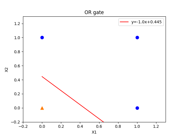 |
| epoch=1546,loss=0.009995,w1=8.515211,w2=8.517734,b=-3.791060 |
| 逻辑与门 AND logic gate |
|---|
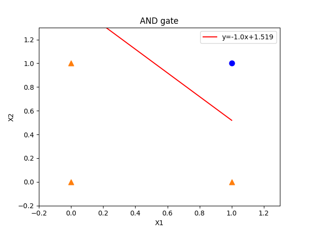 |
| epoch=2872,loss=0.009998,w1=8.537218,w2=8.535023,b=-12.970825 |
###结果分析: *** 通过激活函数将输出值限制在[0,1]之间。两张图中的直线(与门和或门的直线方程)分别将数据点划分成两个区域(0和1)的数据点。直线上方的点的值为1,直线下方的点的值为0。

 浙公网安备 33010602011771号