Hough Transform

目录

• 代码
  • skimage.transform.hough_line

本来想偷懒不记录的, 但是这个Hough Transform实在是有趣.
通过Canny算法等将edge的大体部分检测了出来, 但是往往这些检测出来的点并不是连续的, 那么怎么才能将这些点合理地连接在一起呢?
这个Hough Transform就可以做到这一点. 首先需要明确的一点是, 我们应该将怎么样的点连接起来, 将其中空缺部分的点填补起来? 最简单但是也非常符合直观理解的便是当有多个点处于同一直线的时候, 我们就认为这条线在原图中其实是一个edge.
即对于\(a, b\):

\[y_i = ax_i + b, \quad i=1,2,\cdots. \]

但是每一个点都可以延伸出无数条直线, 对于任意两个条对其连线进行测试是非常耗时耗力的. 这就是Hough Transform的机智的地方.
对于任意一个点, 其都确定了一组线:

\[\tag{line1} b = x_i a - y_i, \]

此构成了\(a, b\)平面上的一条直线, 其上的每一个点都能确定出一条经过点\((x_i, y_i)\)的直线. 对于另一个点\((x_j, y_j)\)可以确定另一条参数直线:

\[\tag{line2} b = x_j a - y_j, \]

显然line1, line2的交点\((a^*, b^*)\)就是由\((x_i, y_i)\)共同确定的直线.
接下来, 我们为图中所有需要关心的点画出其参数直线

\[\tag{line} b = xa - y, \]

线与线之间会产生不同的交点. 根据每个交点所汇聚的直线的数量, 我们就可以判断有多少个点位于同一直线, 且同时将该直线确定出来了.
但是采用(\line)这种表示方式有不便之处, 因为图片\(x, y\)是有0的, 这个会导致我们需要关注的区域是整个平面, 这即便离散化也没有用了. 幸好, 我们还可以用下述方式(类似极坐标)来表示直线:

\[x\cos \theta + y \sin \theta = \rho, \quad \theta \in [-\frac{\pi}{2}, \frac{\pi}{2}]. \]

直观上, \(|\rho|\)是原点到直线距离, 而\(\theta\)是相应的与\(x\)轴所形成的夹角. 图片的原点在左上角, 显然一张\(M \times N\)的图片满足:

\[\rho \in [-\sqrt{M^2 + N^2}, \sqrt{M^2 + N^2}]. \]

所以, 我们只需要关注一个有限的区域即可.
接下来, 我们需要对\(\theta \in [-\frac{\pi}{2}, \frac{\pi}{2}], \rho \in [-\sqrt{M^2 + N^2}, \sqrt{M^2 + N^2}]\)这个区域离散化, 比如取\(\Delta \theta = \frac{\pi}{180}, \Delta \rho = 1\). 对图片中的每一个点\((x, y)\), 根据

\[x\cos \theta + y \sin \theta = \rho, \]

得到:

\[(\theta_1, \rho_1), \cdots, (\theta_{180}, \rho_{180}), \]

并将\(\rho\)四舍五入, 得到:

\[(\theta_1,\mathrm{round}( \rho_1)), \cdots, (\theta_{180}, \mathrm{round} (\rho_{180})), \]

相应的\((\theta, \rho)\)加1, 最后每个\((\theta, \rho)\)处的值就是直线相交的点的个数.

代码

def _hough_lines(img, thetas=None):
    if thetas is None:
        thetas = np.linspace(-np.pi / 2, np.pi / 2, 180)
    the_cos = np.cos(thetas)[..., None]
    the_sin = np.sin(thetas)[..., None]
    x, y = np.where(img > 0) # 源代码用的是 y, x = np.where(img > 0), why?
    lines = (x * the_cos + y * the_sin).T # n x len(thetas)
    return thetas.squeeze(), lines

def hough_transform(img, thetas=None):
    m, n = img.shape
    thetas, lines = _hough_lines(img, thetas)
    offset = int(np.sqrt(m ** 2 + n ** 2)) + 1
    max_distance = offset * 2 + 1
    distances = np.linspace(-offset, offset, max_distance)
    accumulator = np.zeros((max_distance, len(thetas)))
    lines = np.round(lines).astype(np.int32)
    for j in range(len(thetas)):
        for i in lines[:, j]:
            i = i + offset
            accumulator[i, j] += 1
    return accumulator, thetas, distances

import numpy as np
from skimage import io, feature, transform
from freeplot.base import FreePlot
import matplotlib.pyplot as plt

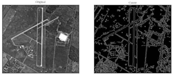
img = io.imread(r"test.png")
img = skimage.color.rgb2gray(img)
fp = FreePlot((1, 2), (8.5, 4), titles=('Original', 'Canny'))
fp.imageplot(img[..., None]) # 0.0.4
edge = skimage.feature.canny(img)
fp.imageplot(edge[..., None], index=(0, 1))
fp.set_title(y=.99)
fp.fig

fp = FreePlot((1, 1), (8, 5))
fp.set_style('no-latex')
thetas, lines, _ = _hough_lines(edge)
x = np.rad2deg(thetas.squeeze())
for i in range(1000):
    y = distances[i]
    fp.lineplot(x, y, alpha=0.01, color='black', style=['line'])

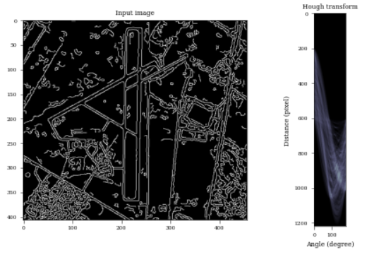
out, angles, d= hough_transform(edge)
fix, axes = plt.subplots(1, 2, figsize=(7, 4))

axes[0].imshow(edge, cmap=plt.cm.gray)
axes[0].set_title('Input image')

axes[1].imshow(
    out, cmap=plt.cm.bone
)
axes[1].set_title('Hough transform')
axes[1].set_xlabel('Angle (degree)')
axes[1].set_ylabel('Distance (pixel)')

plt.tight_layout()
plt.show()

skimage.transform.hough_line

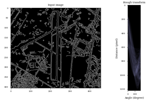
skimage.transform.hough_line

其实我也是参考了hough_line的源代码弄的, 结果是一样的:

out, angles, d = transform.hough_line(edge)

fix, axes = plt.subplots(1, 2, figsize=(7, 4))

axes[0].imshow(edge, cmap=plt.cm.gray)
axes[0].set_title('Input image')

axes[1].imshow(
    out, cmap=plt.cm.bone
)
axes[1].set_title('Hough transform')
axes[1].set_xlabel('Angle (degree)')
axes[1].set_ylabel('Distance (pixel)')

plt.tight_layout()
plt.show()