深度学习网络微调（fine-tune）的基本原理以及应用约束条件 - 以VGG卷积神经网络迁移学习MNIST手写识别任务为例进行的一些实验和总结发现

一、模型预训练通俗理解

0x1：什么是预训练模型（pre-trained model）

预训练模型就是已经用数据集训练好了的模型，这里的数据集一般指大型数据集。比如

VGG16/19
Resnet
Imagenet
COCO

正常情况下，在图像识别任务中常用的VGG16/19等网络是他人调试好的优秀网络，我们无需再修改其网络结构。

参考资料：

https://zhuanlan.zhihu.com/p/35890660
https://github.com/szagoruyko/loadcaffe

0x2：什么是模型微调

用一个单神经元网络解释模型微调的基本原理，

Step1：假设我们的神经网络符合下面的形式：Y = W * X
Step2：现在我们要找到一个W，使得当输入X=2时，输出Y=1，也就是希望W=0.5：1 = W * 2
Step3：按照神经网络的基本训练过程，首先要对W进行初始化，初始化的值符合均值为0，方差为1的分布，假设W初始化为0.1：Y = 0.1 * X
Step4：现在开始训练FP过程，当输入X=2时，W=0.1，输出Y=0.2，这个时候实际值和目标值1的误差为0.8：1 <====== 0.2 = 0.1 * 2
Step5：开始BP反向传导，0.8的误差经过反向传播去更新权值W，假如这次更新为W=0.2，输出位0.4，与目标值的误差为0.6：1 <====== 0.4 = 0.2 * 2
Step6：可能经过10次或20次BP反向传导，W终于得到了我们想要的0.5：Y = 0.5 * X
Step7：如果最开始初始化的时候有人告诉你，W的值应该在0.47附近
Step8：那么从最开始训练，你与目标值的误差就只有0.06了，那么可能只要一步两步BP，就能将W调整到0.5：1 <====== 0.94 = 0.47 * 2

Step7就相当于给你一个预训练模型（pre-trained model），Step8就是基于这个预训练模型去微调（fine-tune）。

可以看到，相对于从头开始训练，微调省去了大量计算资源和计算时间，提高了计算效率，甚至提高了准确率（因为在超大规模训练过程中，模型可能陷入局部次优空间中无法跳出，预训练相当于已经探好了最难的一部分路，后面的路下游模型走起来就轻松了）。

细心的读者可能会注意到，预训练模型对下游fine-tune任务效果的好坏，和以下几个因素有关：

预训练模型训练所用的语料和下游fine-tune任务的重合度：本质上，预训练模型的模型权重参数，代表的是喂入预训练模型的语料。如果预训练任何和下游fine-tune任务领域相差太大，则预训练模型的参数几乎不能起到提效的帮助，甚至可能帮倒忙。
预训练模型自身的容量：理论上，如果预训练模型足够大，能够包含下游任务的一部分核心部分，则预训练模型可以通过权重重调整，在fine-tune的过程中，激活一部分神经元以及关闭一部分神经元，以此使预训练模型朝着下游任务的方向去“生长”。
预训练模型使用的语料库是否足够大和种类丰富，因为这决定了预训练模型是否完成了足够的预训练，否则如果上游预训练模型没有完成收敛，接入下游fine-tune的时候，预训练模型也依然需要进行大量的微调，这对极大拖慢整体模型的收敛。反之，如果预训练模型已经基本完成了收敛，则对下游fine-tune训练的数据集要求就很小，fine-tune就可以基于一个小数据集依然可以得到较好的效果，同时也仅需要较少的训练时间。
预训练模型输入层的向量化方式、张量维度、嵌入方式、编码方位、shape维度等等，和下游fine-tune任务的这些参数结构是否完全一致（或者是否具备一定的迁移性），这里的一致有两方面含义，
- 输入层的一致，理论上说，输入层的结构是一种特征工程的经验形式，它本身也代表了模型对目标任务的某种抽象。打个比方，用于文本生成任务的模型，如果将一个像素图片“强行转换适配”输入进去，最终训练和预测的效果都不会好
- 输出层的一致，输出层的张量维度代表了模型的预测空间，比如一个输出层10维的模型和输出层1000维的模型，它们之间就不具备迁移条件

0x3：为什么要微调？

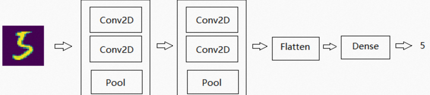
卷积神经网络的核心是：

浅层卷积层提取基础特征，比如边缘，轮廓等基础特征
深层卷积层提取抽象特征，比如整个脸型
全连接层根据特征组合进行评分分类

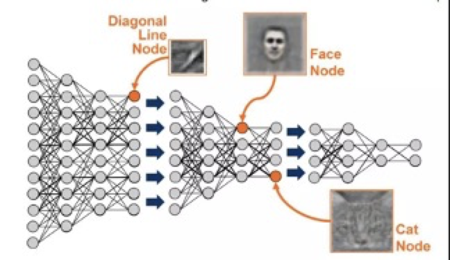
使用大型数据集训练的预训练模型，已经具备了提取浅层基础特征和深层抽象特征的能力。相比不做微调，这种方法具备以下优势：

避免了从头开始训练，减少了训练时间，节省了计算资源
避免了模型不收敛、参数不够优化、准确率低、模型泛化能力低、容易过拟合等问题

0x4：不同数据集下如何进行微调

1、数据量少，但数据相似度非常高

在这种情况下，我们所做的只是修改最后几层或最终的softmax图层的输出类别。

这种情况下，甚至无需fine-tune，可以直接将基模型应用在新的领域任务上。

2、数据量少，数据相似度低

在这种情况下，我们可以冻结预训练模型的初始层（比如k层），并再次训练剩余的（n-k）层。由于新数据集的相似度较低，因此根据新数据集对较高层进行重新训练具有重要意义。

3、数据量大，数据相似度低

在这种情况下，由于我们有一个大的数据集，我们的神经网络训练将会很有效。但是，由于我们的数据与用于训练我们的预训练模型的数据相比有很大不同。使用预训练模型进行的预测不会有效。因此，最好根据你的数据从头开始训练神经网络（Training from scatch）。

4、数据量大，数据相似度高

这是理想情况。在这种情况下，预训练模型应该是最有效的。使用模型的最好方法是保留模型的体系结构和模型的初始权重。然后，我们可以使用在预先训练的模型中的权重来重新训练该模型。

0x5：微调指导事项

通常的做法是截断预先训练好的网络的最后一层（softmax层），并用与我们自己的问题相关的新的softmax层替换它。例如，ImageNet上预先训练好的网络带有1000个类别的softmax图层。如果我们的任务是对10个类别的分类，则网络的新softmax层将由10个类别组成，而不是1000个类别。然后，我们在网络上运行预先训练的权重。确保执行交叉验证，以便网络能够很好地推广。
使用较小的学习率来训练网络。由于我们预计预先训练的权重相对于随机初始化的权重已经相当不错，我们不想过快地扭曲它们太多。通常的做法是使初始学习率比用于从头开始训练（Training from scratch）的初始学习率小10倍。
如果数据集数量过少，我们进来只训练最后一层，如果数据集数量中等，冻结预训练网络的前几层的权重也是一种常见做法。这是因为前几个图层捕捉了与我们的新问题相关的通用特征，如曲线和边。我们希望保持这些权重不变。相反，我们会让网络专注于学习后续深层中特定于数据集的特征。

二、通过卷积核可视化探究fine-tune本质

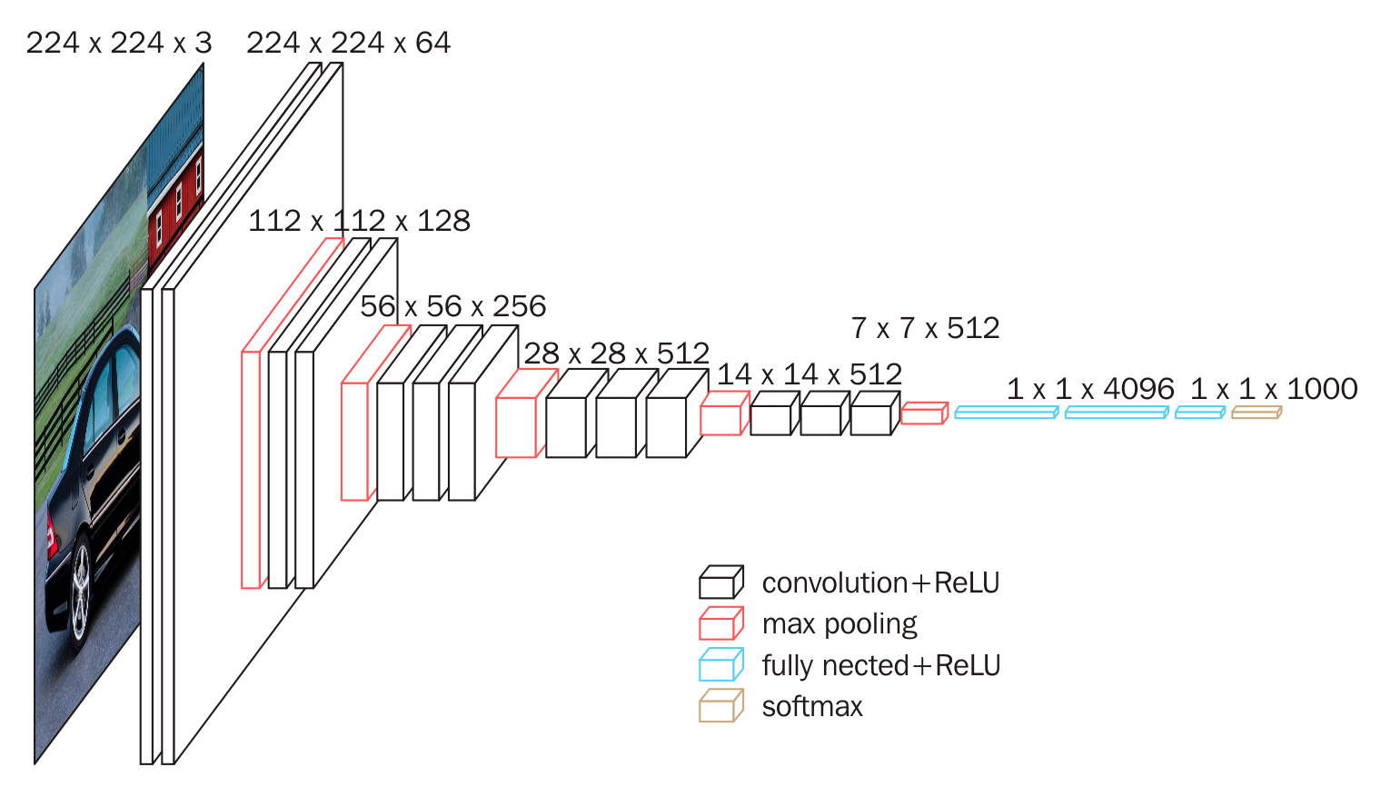
常见的预训练分类网络有牛津的VGG模型、谷歌的Inception模型、微软的ResNet模型等，他们都是预训练的用于分类和检测的卷积神经网络（CNN）。

本次选用的是VGG16模型，是一个在ImageNet数据集上预训练的模型，分类性能优秀，对其他数据集适应能力优秀。

0x1：直接基于VGG16进行手写数字预测

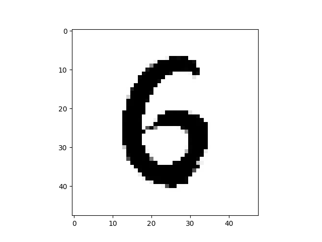
from tensorflow.keras.applications.vgg16 import VGG16
from tensorflow.keras.preprocessing import image
from tensorflow.keras.applications.vgg16 import preprocess_input, decode_predictions
import numpy as np

model = VGG16(weights='imagenet')

img_path = '6.webp'
img = image.load_img(img_path, target_size=(224, 224))
x = image.img_to_array(img)
x = np.expand_dims(x, axis=0)
x = preprocess_input(x)

preds = model.predict(x)
# decode the results into a list of tuples (class, description, probability)
# (one such list for each sample in the batch)
print('Predicted:', decode_predictions(preds, top=3)[0])

6.webp

输出结果：

Predicted: [('n03532672', 'hook', 0.4591384), ('n02910353', 'buckle', 0.032941677), ('n01930112', 'nematode', 0.032439113)]

可以看到，VGG16输出的最高概率预测结果是hook，很明显，VGG16的训练集并没有关于数字图片的样本。

换一个大象图片让VGG16进行识别，

elephant.png

输出结果

Predicted: [('n02504458', 'African_elephant', 0.6726845), ('n01871265', 'tusker', 0.17410518), ('n02504013', 'Indian_elephant', 0.054779347)]

可以看到，VGG16输出的最高概率预测结果是African_elephant，可见VGG16的训练集中是有大象的训练集的，VGG16的卷积层捕获到了大象的线条和外形特征，同时在VGG16的高层也激活了相应的卷积区域感知野。

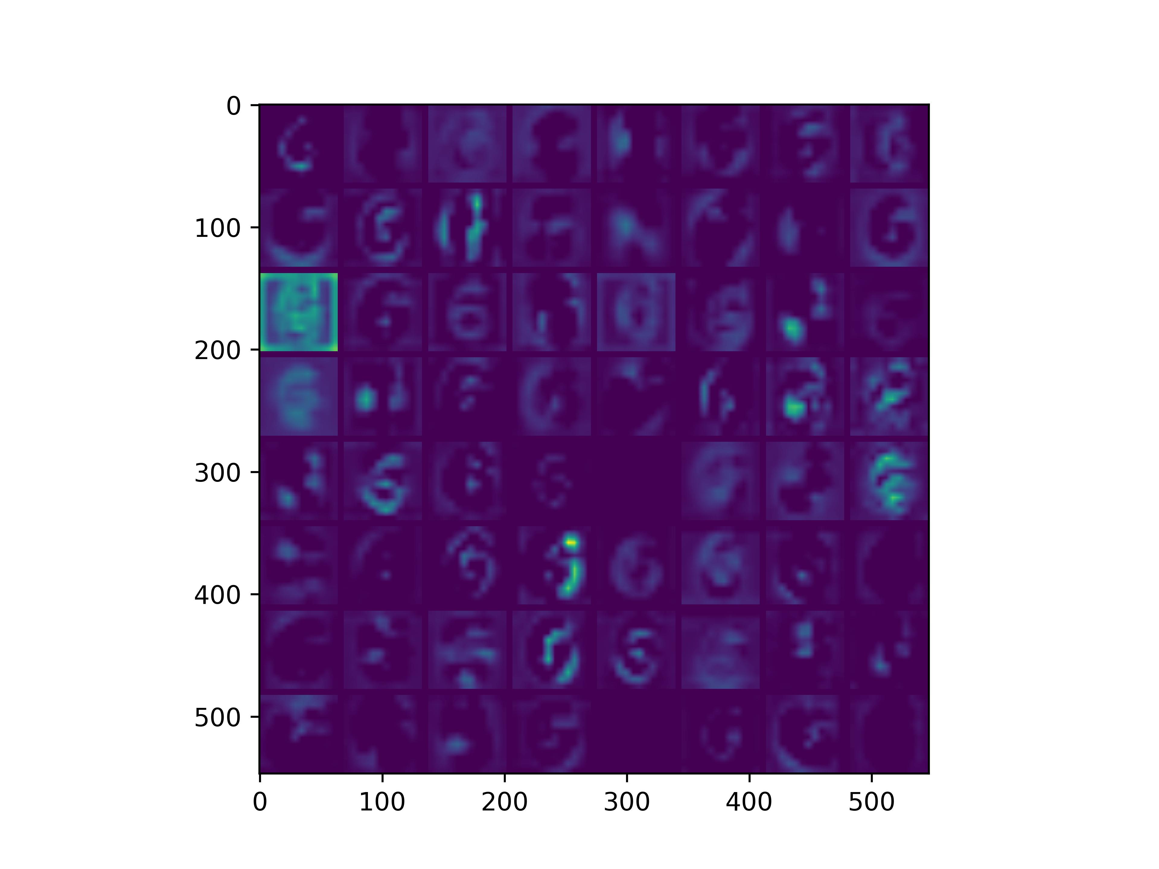
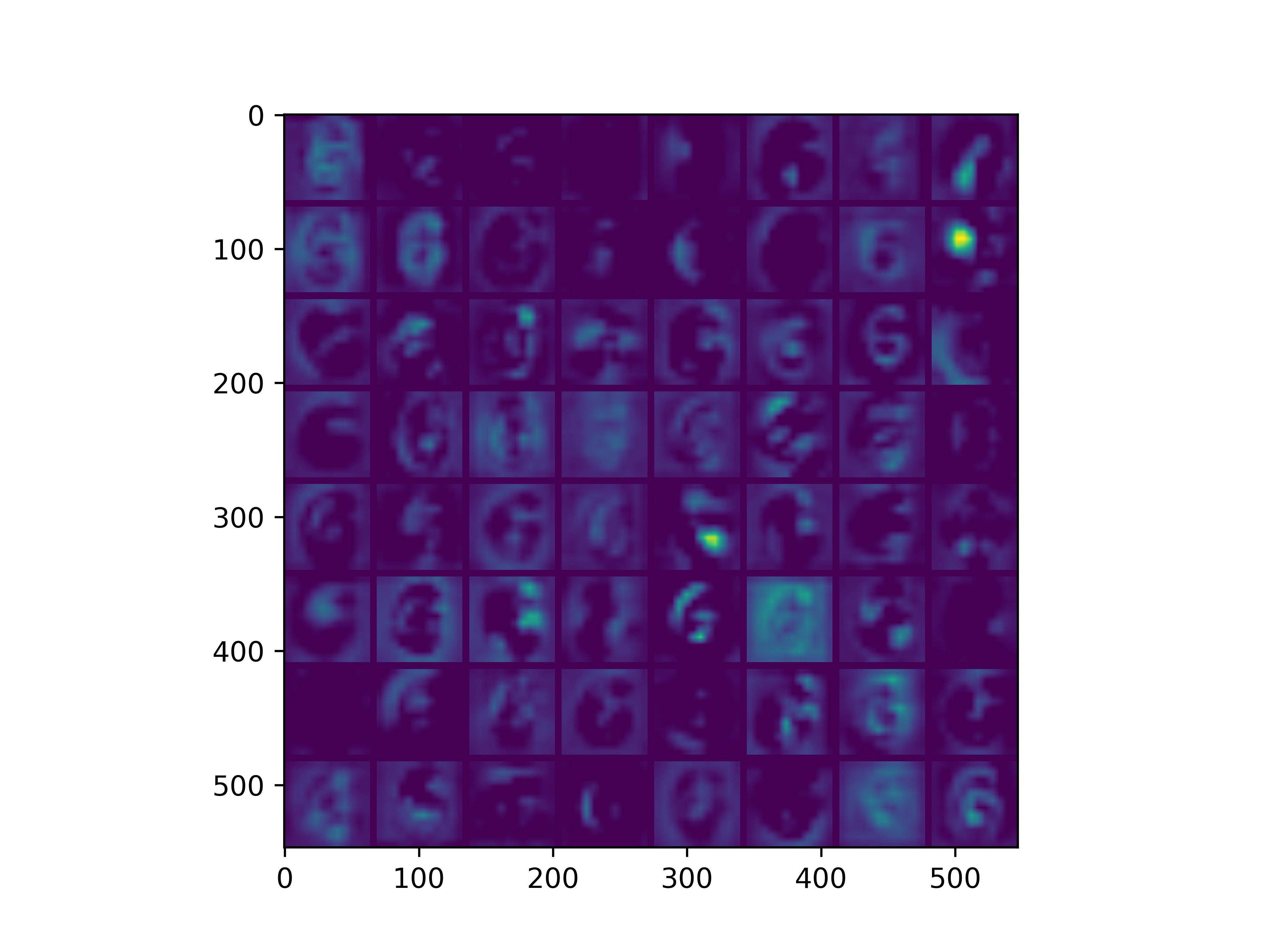
0x2：通过手写数字，可视化VGG16各个层参数

from keras.models import Model
from tensorflow.keras.applications.vgg16 import VGG16
from tensorflow.keras.preprocessing import image
from tensorflow.keras.applications.vgg16 import preprocess_input, decode_predictions
import numpy as np
import cv2
import matplotlib.pyplot as plt


def vis_conv(images, n, name, t):
    """visualize conv output and conv filter.
    Args:
           img: original image.
           n: number of col and row.
           t: vis type.
           name: save name.
    """
    size = 64
    margin = 5

    if t == 'filter':
        results = np.zeros((n * size + 7 * margin, n * size + 7 * margin, 3))
    if t == 'conv':
        results = np.zeros((n * size + 7 * margin, n * size + 7 * margin))

    for i in range(n):
        for j in range(n):
            if t == 'filter':
                filter_img = images[i + (j * n)]
            if t == 'conv':
                filter_img = images[..., i + (j * n)]
            filter_img = cv2.resize(filter_img, (size, size))

            # Put the result in the square `(i, j)` of the results grid
            horizontal_start = i * size + i * margin
            horizontal_end = horizontal_start + size
            vertical_start = j * size + j * margin
            vertical_end = vertical_start + size
            if t == 'filter':
                results[horizontal_start: horizontal_end, vertical_start: vertical_end, :] = filter_img
            if t == 'conv':
                results[horizontal_start: horizontal_end, vertical_start: vertical_end] = filter_img

    # Display the results grid
    plt.imshow(results)
    plt.savefig('images/{}_{}.jpg'.format(t, name), dpi=600)
    plt.show()


def conv_output(model, layer_name, img):
    """Get the output of conv layer.

    Args:
           model: keras model.
           layer_name: name of layer in the model.
           img: processed input image.

    Returns:
           intermediate_output: feature map.
    """
    # this is the placeholder for the input images
    input_img = model.input

    try:
        # this is the placeholder for the conv output
        out_conv = model.get_layer(layer_name).output
    except:
        raise Exception('Not layer named {}!'.format(layer_name))

    # get the intermediate layer model
    intermediate_layer_model = Model(inputs=input_img, outputs=out_conv)

    # get the output of intermediate layer model
    intermediate_output = intermediate_layer_model.predict(img)

    return intermediate_output[0]


if __name__ == '__main__':
    model = VGG16(weights='imagenet')

    img_path = '6.webp'
    img = image.load_img(img_path, target_size=(224, 224))
    x = image.img_to_array(img)
    x = np.expand_dims(x, axis=0)
    x = preprocess_input(x)

    preds = model.predict(x)
    # decode the results into a list of tuples (class, description, probability)
    # (one such list for each sample in the batch)
    print('Predicted:', decode_predictions(preds, top=3)[0])

    conv_output_block1_conv1 = conv_output(model, "block1_conv1", x)
    print("block1_conv1: ", conv_output_block1_conv1)
    vis_conv(conv_output_block1_conv1, 8, "block1_conv1", 'conv')

    conv_output_block1_conv2 = conv_output(model, "block1_conv2", x)
    print("block1_conv2: ", conv_output_block1_conv2)
    vis_conv(conv_output_block1_conv2, 8, "block1_conv2", 'conv')

    conv_output_block2_conv1 = conv_output(model, "block2_conv1", x)
    print("block2_conv1: ", conv_output_block2_conv1)
    vis_conv(conv_output_block2_conv1, 8, "block2_conv1", 'conv')

    conv_output_block2_conv2 = conv_output(model, "block2_conv2", x)
    print("block2_conv2: ", conv_output_block2_conv2)
    vis_conv(conv_output_block2_conv2, 8, "block2_conv2", 'conv')

    conv_output_block3_conv1 = conv_output(model, "block3_conv1", x)
    print("block3_conv1: ", conv_output_block3_conv1)
    vis_conv(conv_output_block3_conv1, 8, "block3_conv1", 'conv')

    conv_output_block3_conv2 = conv_output(model, "block3_conv2", x)
    print("block3_conv2: ", conv_output_block3_conv2)
    vis_conv(conv_output_block3_conv2, 8, "block3_conv2", 'conv')

    conv_output_block5_conv3 = conv_output(model, "block5_conv3", x)
    print("block5_conv3: ", conv_output_block5_conv3)
    vis_conv(conv_output_block5_conv3, 8, "block5_conv3", 'conv')

    print("fc1: ", conv_output(model, "fc1", x))
    print("fc2: ", conv_output(model, "fc2", x))
    print("predictions: ", conv_output(model, "predictions", x))

View Code

输出结果：

1/1 [==============================] - 2s 2s/step
Predicted: [('n03532672', 'hook', 0.4591384), ('n02910353', 'buckle', 0.032941677), ('n01930112', 'nematode', 0.032439113)]
1/1 [==============================] - 0s 53ms/step
block1_conv1:  [[[  0.         42.11969     0.        ...   0.         32.04823
     0.       ]
  [  0.         46.303555   82.50592   ...   0.        324.38284
   164.56157  ]
  [  0.         46.303555   82.50592   ...   0.        324.38284
   164.56157  ]
  ...
  [  0.         46.303555   82.50592   ...   0.        324.38284
   164.56157  ]
  [  0.         46.303555   82.50592   ...   0.        324.38284
   164.56157  ]
  [  2.61003    32.20762   173.75212   ...   0.        517.4678
   391.77734  ]]

 [[  0.         56.784718    0.        ...   0.          0.
     0.       ]
  [  2.401019   58.89123    63.275116  ...   0.          2.2158926
    10.105784 ]
  [  2.401019   58.89123    63.275116  ...   0.          2.2158926
    10.105784 ]
  ...
  [  2.401019   58.89123    63.275116  ...   0.          2.2158926
    10.105784 ]
  [  2.401019   58.89123    63.275116  ...   0.          2.2158926
    10.105784 ]
  [377.4901     38.781555  204.19121   ...   0.        382.94656
   378.29724  ]]

 [[  0.         56.784718    0.        ...   0.          0.
     0.       ]
  [  2.401019   58.89123    63.275116  ...   0.          2.2158926
    10.105784 ]
  [  2.401019   58.89123    63.275116  ...   0.          2.2158926
    10.105784 ]
  ...
  [  2.401019   58.89123    63.275116  ...   0.          2.2158926
    10.105784 ]
  [  2.401019   58.89123    63.275116  ...   0.          2.2158926
    10.105784 ]
  [377.4901     38.781555  204.19121   ...   0.        382.94656
   378.29724  ]]

 ...

 [[  0.         56.784718    0.        ...   0.          0.
     0.       ]
  [  2.401019   58.89123    63.275116  ...   0.          2.2158926
    10.105784 ]
  [  2.401019   58.89123    63.275116  ...   0.          2.2158926
    10.105784 ]
  ...
  [  2.401019   58.89123    63.275116  ...   0.          2.2158926
    10.105784 ]
  [  2.401019   58.89123    63.275116  ...   0.          2.2158926
    10.105784 ]
  [377.4901     38.781555  204.19121   ...   0.        382.94656
   378.29724  ]]

 [[  0.         56.784718    0.        ...   0.          0.
     0.       ]
  [  2.401019   58.89123    63.275116  ...   0.          2.2158926
    10.105784 ]
  [  2.401019   58.89123    63.275116  ...   0.          2.2158926
    10.105784 ]
  ...
  [  2.401019   58.89123    63.275116  ...   0.          2.2158926
    10.105784 ]
  [  2.401019   58.89123    63.275116  ...   0.          2.2158926
    10.105784 ]
  [377.4901     38.781555  204.19121   ...   0.        382.94656
   378.29724  ]]

 [[  0.         39.011864    0.        ...   0.          0.
     0.       ]
  [323.5314     39.00029    97.09346   ...   0.          0.
    67.22728  ]
  [323.5314     39.00029    97.09346   ...   0.          0.
    67.22728  ]
  ...
  [323.5314     39.00029    97.09346   ...   0.          0.
    67.22728  ]
  [323.5314     39.00029    97.09346   ...   0.          0.
    67.22728  ]
  [523.7337     25.070164  184.00014   ...   0.        144.83621
   315.41928  ]]]
1/1 [==============================] - 0s 84ms/step
block1_conv2:  [[[982.48444    65.59724     0.        ...  81.02978   698.99084
   172.65338  ]
  [256.9937    101.16306     8.7225065 ... 203.38603   340.56735
     0.       ]
  [314.77548   126.94779     0.        ... 159.34764   175.0137
     0.       ]
  ...
  [314.77548   126.94779     0.        ... 159.34764   175.0137
     0.       ]
  [ 63.2487      0.          0.        ... 125.09357   413.46884
    33.402287 ]
  [  0.          0.          0.        ...  32.059208    0.
     7.143284 ]]

 [[401.39062    97.3492      0.        ... 134.1313    454.73416
     0.       ]
  [  0.         97.926704  136.89134   ... 259.61768   632.9747
     0.       ]
  [  0.        125.44156    95.91204   ... 174.20306   390.24847
     0.       ]
  ...
  [  0.        125.44156    95.91204   ... 174.20306   390.24847
     0.       ]
  [  0.          0.        109.98622   ... 103.348114  854.354
     0.       ]
  [  0.          0.          0.        ...   0.        394.38068
     0.       ]]

 [[396.95483   167.3767      0.        ...  69.25613   207.11255
     4.1853294]
  [  0.        174.81584    76.58766   ... 161.11617   339.40433
     0.       ]
  [151.61284    87.23442    16.130083  ...   6.742235    1.1302795
     0.       ]
  ...
  [151.61284    87.23442    16.130083  ...   6.742235    1.1302795
     0.       ]
  [  0.          0.         70.19446   ...   0.        479.9812
   254.07501  ]
  [  0.          0.          0.        ...   0.        199.8518
    50.87436  ]]

 ...

 [[396.95483   167.3767      0.        ...  69.25613   207.11255
     4.1853294]
  [  0.        174.81584    76.58766   ... 161.11617   339.40433
     0.       ]
  [151.61284    87.23442    16.130083  ...   6.742235    1.1302795
     0.       ]
  ...
  [151.61284    87.23442    16.130083  ...   6.742235    1.1302795
     0.       ]
  [  0.          0.         70.19446   ...   0.        479.9812
   254.07501  ]
  [  0.          0.          0.        ...   0.        199.8518
    50.87436  ]]

 [[196.74297     0.          0.        ...  76.20704   371.12302
   239.03537  ]
  [  0.          0.         54.11582   ... 132.80391   642.51025
   472.34528  ]
  [  0.          0.          4.422485  ...   7.28855   283.40457
   706.94666  ]
  ...
  [  0.          0.          4.422485  ...   7.28855   283.40457
   706.94666  ]
  [  0.          0.         54.947617  ...   0.        688.73157
   731.2318   ]
  [  0.          0.          0.        ...   0.        364.4021
   284.65625  ]]

 [[  0.          0.          0.        ...   0.          0.
     0.       ]
  [  0.          0.          0.        ...   0.        407.869
     0.       ]
  [  0.          0.          0.        ...   0.        198.98882
   101.46747  ]
  ...
  [  0.          0.          0.        ...   0.        198.98882
   101.46747  ]
  [  0.          0.          0.        ...   0.        534.15466
    69.81046  ]
  [287.62454     0.          0.        ...   0.        764.0485
     0.       ]]]
1/1 [==============================] - 0s 76ms/step
block2_conv1:  [[[   0.          0.        146.08685  ... 1138.9917      0.
   1914.1439  ]
  [   0.          0.        617.18994  ...  630.32166     0.
      0.      ]
  [   0.          0.        479.59012  ...  803.52374     0.
    281.59882 ]
  ...
  [   0.          0.        479.59012  ...  803.52374     0.
    281.59882 ]
  [   0.          0.        583.4128   ...  895.7679      0.
    715.7333  ]
  [   0.          0.       1087.817    ... 2163.6226      0.
      0.      ]]

 [[   0.        657.53296     0.       ...  660.99      461.2479
   1719.0864  ]
  [   0.        823.556     349.60562  ...    0.        542.6992
      0.      ]
  [   0.        748.83795   131.92645  ...   30.981398  517.1108
     82.481895]
  ...
  [   0.        748.83795   131.92645  ...   30.981398  517.1108
     82.481895]
  [   0.        826.5497    252.64777  ...   64.045074  392.9257
    619.41876 ]
  [   0.        693.9135   1073.2073   ... 1989.0895    697.90814
      0.      ]]

 [[   0.        239.73143     0.       ...  901.56885   274.7921
   1343.2406  ]
  [   0.        214.44774   181.45721  ...    0.        279.94656
      0.      ]
  [   0.        130.28665     0.       ...   90.52182   205.50911
    130.00967 ]
  ...
  [   0.        130.28665     0.       ...   90.52182   205.50911
    130.00967 ]
  [   0.        230.28584    60.274647 ...   54.528107   35.845345
    758.34717 ]
  [   0.        283.4764    837.31805  ... 1669.6423    417.16782
    390.9171  ]]

 ...

 [[   0.        239.73143     0.       ...  901.56885   274.7921
   1343.2406  ]
  [   0.        214.44774   181.45721  ...    0.        279.94656
      0.      ]
  [   0.        130.28665     0.       ...   90.52182   205.50911
    130.00967 ]
  ...
  [   0.        130.28665     0.       ...   90.52182   205.50911
    130.00967 ]
  [   0.        230.28584    60.274647 ...   54.528107   35.845345
    758.34717 ]
  [   0.        283.4764    837.31805  ... 1669.6423    417.16782
    390.9171  ]]

 [[   0.        149.2003      0.       ...  467.1346    130.91127
   1713.3496  ]
  [   0.         89.11      283.70944  ...    0.        236.00652
      0.      ]
  [   0.         21.128517   52.216312 ...    0.        233.49413
     93.75622 ]
  ...
  [   0.         21.128517   52.216312 ...    0.        233.49413
     93.75622 ]
  [   0.        120.84711   171.13362  ...    0.         73.68687
    632.3945  ]
  [   0.        207.82211   976.44196  ... 1907.8083    525.08185
     29.64562 ]]

 [[   0.        296.92758   171.61426  ...  975.3303    292.51434
   1616.5455  ]
  [   0.        235.07794   710.6981   ...  276.39038     0.
      0.      ]
  [   0.        116.03024   512.0845   ...  650.45764    53.27237
    331.76382 ]
  ...
  [   0.        116.03024   512.0845   ...  650.45764    53.27237
    331.76382 ]
  [   0.        247.85234   603.1937   ...  753.06476    57.02111
    653.146   ]
  [   0.        435.59036  1229.345    ... 2149.0642    365.4059
      0.      ]]]
WARNING:tensorflow:5 out of the last 5 calls to <function Model.make_predict_function.<locals>.predict_function at 0x7ff36c074790> triggered tf.function retracing. Tracing is expensive and the excessive number of tracings could be due to (1) creating @tf.function repeatedly in a loop, (2) passing tensors with different shapes, (3) passing Python objects instead of tensors. For (1), please define your @tf.function outside of the loop. For (2), @tf.function has reduce_retracing=True option that can avoid unnecessary retracing. For (3), please refer to https://www.tensorflow.org/guide/function#controlling_retracing and https://www.tensorflow.org/api_docs/python/tf/function for  more details.
1/1 [==============================] - 0s 96ms/step
block2_conv2:  [[[  19.134865   65.2908    388.85107  ...   77.567345    0.
      0.      ]
  [ 385.78787     0.         83.92136  ...  823.738       0.
      0.      ]
  [ 362.76718     0.          0.       ...  770.1545      0.
      0.      ]
  ...
  [ 370.19595     0.          0.       ...  693.7316      0.
      0.      ]
  [ 395.07098  1163.4445      0.       ...  685.89105     0.
      0.      ]
  [ 393.64594   221.8914      0.       ...  779.5206      0.
      0.      ]]

 [[   0.          0.        658.96985  ...  266.29254  1334.6693
      0.      ]
  [ 175.15945     0.          0.       ...  927.1358    410.14014
      0.      ]
  [ 113.65867     0.          0.       ...  705.73663   115.82475
    341.95673 ]
  ...
  [  89.81759   278.56213     0.       ...  651.8543    775.20416
    502.7654  ]
  [ 136.82233  1937.8406      0.       ...  647.9445    302.8629
    525.4279  ]
  [ 262.19644   357.42938     0.       ...  750.1874      0.
    489.33453 ]]

 [[   0.          0.        418.21606  ...   12.688118  795.45483
      0.      ]
  [ 234.67218     0.          0.       ...  426.10312     0.
      0.      ]
  [ 145.08507     0.          0.       ...  287.3707      0.
    296.64294 ]
  ...
  [ 103.087685  305.11697    62.120567 ...  267.3017    545.9968
    524.84625 ]
  [ 235.22937  2067.736     239.66722  ...  172.1788    407.2032
    489.35236 ]
  [ 323.7679    407.43408   319.0578   ...  341.47412     0.
    345.82104 ]]

 ...

 [[   0.          0.        580.24994  ...   68.54731   589.51636
      0.      ]
  [ 201.64163     0.        157.14062  ...  501.0832      0.
      0.      ]
  [ 133.07848     0.          0.       ...  351.53003     0.
    415.4161  ]
  ...
  [  86.24023   465.5442     22.741163 ...  337.74213   215.66536
    622.05804 ]
  [ 174.42499  2174.4937     46.142918 ...  286.23798   212.43034
    572.5916  ]
  [ 282.7715    504.28677   132.34572  ...  501.6414      0.
    371.98062 ]]

 [[   0.          0.        247.89134  ...  337.7562    870.8283
      0.      ]
  [ 129.28552     0.          0.       ...  976.0519      0.
      0.      ]
  [   0.        107.290855    0.       ...  696.99493     0.
    248.08282 ]
  ...
  [   0.        545.71716     0.       ...  687.88995   175.53624
    456.3958  ]
  [  40.394768 2056.4695      0.       ...  716.48956   157.10045
    438.98425 ]
  [ 169.84534   324.61182   357.57187  ...  724.79034     0.
    279.55737 ]]

 [[   0.          0.          0.       ...  108.35586  1594.9191
      0.      ]
  [   0.          0.          0.       ...  641.5959    631.3734
      0.      ]
  [   0.          0.          0.       ...  476.7445    236.77658
      0.      ]
  ...
  [   0.          0.          0.       ...  514.81213   659.1744
      0.      ]
  [   0.        558.51337     0.       ...  529.3481    646.179
      0.      ]
  [   0.          0.        318.3686   ...  567.25116     0.
     85.41164 ]]]
WARNING:tensorflow:6 out of the last 6 calls to <function Model.make_predict_function.<locals>.predict_function at 0x7ff36c0250d0> triggered tf.function retracing. Tracing is expensive and the excessive number of tracings could be due to (1) creating @tf.function repeatedly in a loop, (2) passing tensors with different shapes, (3) passing Python objects instead of tensors. For (1), please define your @tf.function outside of the loop. For (2), @tf.function has reduce_retracing=True option that can avoid unnecessary retracing. For (3), please refer to https://www.tensorflow.org/guide/function#controlling_retracing and https://www.tensorflow.org/api_docs/python/tf/function for  more details.
1/1 [==============================] - 0s 86ms/step
block3_conv1:  [[[ 104.03467     0.       7676.7437   ...  284.6595    104.21471
    495.0637  ]
  [   0.        313.47745  5637.235    ...  773.39124   312.671
    710.7272  ]
  [   0.        626.0542   4799.9775   ...  797.72      329.52908
    588.2553  ]
  ...
  [   0.        646.8998   4819.6846   ...  770.5025    316.77924
    555.9198  ]
  [   0.        247.11465  5635.4976   ...  528.78986   281.3929
    570.0344  ]
  [  30.971907    0.       7807.489    ...  149.22829   247.03853
    569.7642  ]]

 [[   0.        871.3891   5385.873    ...  138.57967   142.74121
    983.03674 ]
  [   0.       1012.0134    499.58597  ...  162.09428   256.54013
   1158.3336  ]
  [   0.       1021.0573     28.230726 ...  184.61717   219.79193
    785.92285 ]
  ...
  [   0.       1050.2477      0.       ...  146.40399   266.05975
    744.28723 ]
  [   0.        998.98596   374.99014  ...   64.251434  274.85852
    940.72205 ]
  [   0.        715.7788   5695.999    ...  181.9697    113.495964
    998.7362  ]]

 [[   0.        715.5003   4931.604    ...  174.02486   218.0967
    733.6579  ]
  [   0.        782.053      98.879425 ...  201.88213   215.22943
    785.8126  ]
  [   0.        754.37915     0.       ...  156.65364    84.32829
    489.68857 ]
  ...
  [   0.        784.71075     0.       ...  119.22443   137.86731
    454.97656 ]
  [   0.        741.68567     0.       ...   42.16644   243.78513
    592.8224  ]
  [   0.        564.874    5148.9604   ...  128.61302   147.20853
    733.89886 ]]

 ...

 [[   0.        496.68298  4885.435    ...  318.65524   245.03665
    575.7172  ]
  [   0.        486.5161     27.83389  ...  512.1368    232.01933
    566.13635 ]
  [   0.        477.45157     0.       ...  499.04877    68.24934
    263.7914  ]
  ...
  [   0.        499.77722     0.       ...  459.50702   132.83049
    226.18076 ]
  [   0.        439.5999      0.       ...  320.2604    207.68942
    371.76605 ]
  [   0.        339.14404  5100.4336   ...  253.7242    112.67809
    590.3231  ]]

 [[   0.        347.25443  5573.7017   ...  627.8705    275.148
    631.8805  ]
  [   0.        358.82916   292.3079   ...  979.4485    303.31757
    662.5002  ]
  [   0.        478.66336     0.       ... 1011.04913   144.6257
    358.16284 ]
  ...
  [   0.        500.74857     0.       ...  972.3128    223.55475
    336.5134  ]
  [   0.        355.48328   104.18472  ...  832.22375   270.79025
    496.9038  ]
  [   0.        219.11375  5712.4497   ...  539.98773    84.06546
    667.78613 ]]

 [[   0.        604.2773   7762.388    ...  492.06854   294.44586
    373.23422 ]
  [   0.        660.0235   5493.3257   ...  210.03978   176.89102
    304.05936 ]
  [   0.        675.077    4603.5874   ...  169.29701   125.09003
     53.69849 ]
  ...
  [   0.        701.2141   4594.911    ...  142.22992   227.38722
     59.698753]
  [   0.        718.4968   5527.42     ...  161.2458    129.69702
    249.47922 ]
  [   0.        586.12274  8277.507    ...  435.10352     0.
    348.29013 ]]]
1/1 [==============================] - 0s 105ms/step
block3_conv2:  [[[   0.        971.66376   794.8841   ...  172.1506     10.597431
    794.8708  ]
  [   0.        291.7925    826.4213   ...   39.319454    0.
    718.3281  ]
  [   0.        156.54356   802.0568   ...    0.          0.
    503.39447 ]
  ...
  [   0.        401.88135  1241.3585   ...    0.          0.
    362.15497 ]
  [   0.        675.3719   1448.097    ...    0.          9.820769
    410.58932 ]
  [   0.         10.890532  953.4981   ...  233.22906     0.
    579.7396  ]]

 [[ 575.767    1863.7603    592.8948   ...  245.05453     0.
   1068.8091  ]
  [ 514.8801    844.0041    222.19751  ...    0.          0.
    788.1397  ]
  [  19.14704   444.27817   111.57798  ...    0.          0.
    409.57492 ]
  ...
  [ 252.99167   848.908     513.1679   ...    0.          0.
    312.90305 ]
  [ 591.92786  1448.2924    630.19824  ...    0.          0.
    504.8597  ]
  [   0.        379.8196    763.054    ...    0.         72.78092
    733.65424 ]]

 [[ 287.43423  1910.7128    349.80966  ...  387.3527      0.
   1265.1278  ]
  [   0.        740.3088    124.85873  ...    0.          0.
    918.3699  ]
  [   0.        286.83832   118.424774 ...    0.        177.10791
    486.00412 ]
  ...
  [   0.        735.8566    558.8175   ...    0.        193.26689
    449.90454 ]
  [  53.59411  1525.2466    651.7935   ...    0.        103.276146
    716.995   ]
  [   0.        603.8922    836.88104  ...   50.30762   191.5637
    884.57367 ]]

 ...

 [[ 292.4923   1834.398     444.55945  ...  540.1754     14.972595
   1457.0437  ]
  [   0.        642.0181    319.91138  ...   44.719204  156.22743
   1106.5459  ]
  [   0.        170.11359   338.21768  ...    0.        376.42972
    603.82666 ]
  ...
  [   0.        581.471     737.77203  ...    0.        400.47705
    579.5313  ]
  [   0.       1367.3385    798.4122   ...    0.        260.49323
    826.0262  ]
  [   0.        544.79816   826.0728   ...   77.14375   283.54224
    990.2182  ]]

 [[ 584.30676  1950.905     596.8577   ...  740.97327    81.50432
   1820.6097  ]
  [ 116.4952    835.781     588.2435   ...  225.01852   196.70117
   1720.8013  ]
  [   0.        356.6451    615.6922   ...   77.022446  354.97284
   1198.3191  ]
  ...
  [   0.        733.50824  1012.90985  ...    0.        296.32776
   1099.1088  ]
  [ 186.0945   1339.9901   1179.6779   ...    0.        191.2773
   1315.7777  ]
  [   0.        384.91098  1044.8905   ...  228.41646   209.99303
   1404.8423  ]]

 [[ 608.40894  1603.2566    899.59283  ...  999.1029     64.82636
   1448.8973  ]
  [ 733.8801   1092.808     762.7826   ...  444.4963    137.76027
   1666.6692  ]
  [ 293.81265   823.8305    784.1011   ...  267.9691    135.08733
   1363.0045  ]
  ...
  [ 359.85425  1058.6151   1013.9297   ...  163.37076   159.4037
   1266.5629  ]
  [ 682.56195  1274.0765   1125.9093   ...  177.28194   135.8132
   1424.4539  ]
  [ 148.46483   454.86966   954.3874   ...  199.56137   320.5976
   1351.9453  ]]]
1/1 [==============================] - 0s 146ms/step
block5_conv3:  [[[0.        0.        0.        ... 0.        0.        0.       ]
  [0.        0.        0.        ... 0.        0.        0.       ]
  [0.        0.        0.        ... 0.        0.        0.       ]
  ...
  [0.        0.        0.        ... 0.        0.        0.       ]
  [0.        0.        0.        ... 0.        0.        0.       ]
  [0.        0.        0.        ... 0.        0.        0.       ]]

 [[0.        0.        0.        ... 0.        0.        0.       ]
  [0.        0.        0.        ... 0.        0.        0.       ]
  [0.        0.        0.        ... 0.        0.        0.       ]
  ...
  [0.        0.        0.        ... 0.        0.        0.       ]
  [0.        0.        0.        ... 0.        0.        0.       ]
  [0.        0.        0.        ... 0.        0.        0.       ]]

 [[0.        0.        0.        ... 0.        0.        0.       ]
  [0.        0.        0.        ... 0.        0.        0.       ]
  [0.        0.        0.        ... 0.        0.        0.       ]
  ...
  [0.        0.        0.        ... 0.        0.        0.       ]
  [0.        0.        0.        ... 0.        0.        0.       ]
  [0.        0.        0.        ... 0.        0.        0.       ]]

 ...

 [[0.        0.        0.        ... 0.        0.        0.       ]
  [0.        0.        0.        ... 0.        0.        0.       ]
  [0.        0.        0.        ... 0.        1.2440066 0.       ]
  ...
  [0.        0.        0.        ... 0.        0.        0.       ]
  [0.        0.        0.        ... 0.        0.        0.       ]
  [0.        0.        0.        ... 0.        0.        0.       ]]

 [[0.        0.        0.        ... 0.        0.        0.       ]
  [0.        0.        0.        ... 0.        0.        0.       ]
  [0.        0.        0.        ... 0.        0.        0.       ]
  ...
  [0.        0.        0.        ... 0.        0.        0.       ]
  [0.        0.        0.        ... 0.        0.        0.       ]
  [0.        0.        0.        ... 0.        0.        0.       ]]

 [[0.        0.        0.        ... 0.        0.        0.       ]
  [0.        0.        0.        ... 0.        0.        0.       ]
  [0.        0.        0.        ... 0.        0.5987776 0.       ]
  ...
  [0.        0.        0.        ... 0.        0.        0.       ]
  [0.        0.        0.        ... 0.        0.        0.       ]
  [0.        0.        0.        ... 0.        0.        0.       ]]]
1/1 [==============================] - 0s 138ms/step
fc1:  [2.9445024  0.         0.         ... 3.411133   0.         0.92348397]
1/1 [==============================] - 0s 143ms/step
fc2:  [0.         0.         0.         ... 0.01487154 0.         0.        ]
1/1 [==============================] - 0s 153ms/step
predictions:  [8.86679481e-06 3.92886477e-06 1.90436788e-06 1.05222316e-05
 2.95820100e-05 1.05888921e-05 8.18475996e-07 2.97174847e-05
 1.72565160e-05 2.33364801e-04 4.08327742e-06 7.54527573e-05
 2.13582698e-05 5.62608966e-06 2.66997467e-05 6.33711488e-06
 5.91164498e-05 2.96048438e-05 1.54325113e-04 1.61606149e-04
 4.36949313e-06 2.27579949e-04 3.22062464e-04 3.87774286e-04
 1.82932072e-05 1.78626142e-04 1.06591207e-04 1.24504077e-04
 7.32575209e-05 1.67771868e-05 1.42938734e-06 5.67790994e-06
 4.40411623e-06 3.51705899e-06 4.54849214e-06 8.11457880e-07
 1.23381051e-06 9.66434072e-07 1.74248067e-04 4.33074547e-06
 3.25646602e-06 1.54293630e-05 1.26219347e-05 1.96861256e-05
 5.53511854e-05 5.12993356e-05 5.80043570e-06 9.02399624e-05
 7.22741834e-06 1.27374151e-05 2.59617846e-05 3.38299797e-05
 2.39712815e-03 1.74616615e-03 4.85557830e-04 3.29024158e-04
 3.13818571e-04 2.12321938e-05 5.26380085e-04 2.88680475e-03
 1.84028875e-03 8.09462945e-05 6.80478770e-05 2.14936007e-02
 3.19925428e-04 1.66888710e-03 2.04587798e-03 3.49455629e-04
 1.27097068e-03 2.72739620e-04 2.91247284e-06 4.48031962e-04
 1.57972545e-06 7.40459245e-06 1.13488693e-06 9.91967318e-06
 1.07233291e-05 1.95666644e-06 1.85278812e-04 3.24987195e-04
 5.19032947e-05 2.71407112e-06 1.49551488e-05 4.88938567e-05
 5.17146982e-05 1.10298810e-04 1.06869438e-05 2.46440832e-05
 4.66025049e-05 3.63443614e-05 1.12969128e-05 2.55341893e-05
 6.81859092e-05 1.14550072e-04 5.32956028e-06 7.00814735e-06
 1.15207583e-03 1.13513424e-05 1.45131880e-05 9.87223932e-04
 1.41433545e-03 1.42524106e-04 1.87630758e-05 1.45034219e-05
 7.02911166e-06 4.97291239e-07 1.44432697e-05 2.14918982e-05
 2.49657751e-04 1.75241279e-04 7.07811036e-04 3.24391127e-02
 2.39375167e-05 4.87557236e-06 1.68786224e-04 1.72599885e-05
 3.57204262e-04 3.65287306e-05 9.62294143e-06 6.66444794e-06
 6.23000451e-05 4.13392627e-05 1.25281904e-05 2.46514765e-06
 1.16787705e-05 4.36370010e-06 1.15267576e-05 1.03567043e-04
 1.90633407e-04 5.81696622e-06 5.24300151e-04 4.73948821e-05
 6.00396706e-05 2.62725348e-06 9.41229882e-06 4.48861829e-05
 3.18245611e-06 1.09500215e-05 3.04656010e-06 2.81243956e-06
 2.78029938e-06 2.36011829e-06 1.19211859e-06 1.40344800e-05
 6.92425092e-05 2.19969384e-04 2.38212277e-04 5.18192837e-06
 6.66403794e-05 1.19804699e-05 1.12324997e-05 7.82153511e-05
 1.48655672e-05 7.67800702e-06 3.79271878e-05 9.57871907e-06
 1.36488925e-05 9.52548271e-06 1.79516901e-05 3.11920776e-05
 1.07268534e-04 2.04860935e-05 1.13185033e-05 4.38859715e-05
 6.85368195e-06 3.27570451e-05 4.21883669e-06 9.13747954e-06
 1.15643152e-05 7.98587553e-06 9.62191461e-06 2.23533661e-05
 1.18041371e-05 4.75581110e-05 6.63245373e-06 3.38082427e-05
 9.82034999e-06 2.01295570e-05 8.89091098e-06 2.23101542e-05
 2.10599119e-05 1.95221619e-05 2.93983067e-05 1.35727038e-04
 4.10272987e-05 9.92941568e-05 8.58638596e-05 4.45206533e-05
 7.41288459e-05 4.27207560e-05 7.12208493e-05 1.87339421e-04
 5.40639439e-06 6.58450299e-05 7.53286349e-06 1.91383544e-04
 1.07185342e-05 3.62894643e-05 1.38193327e-05 3.58770776e-05
 9.85885981e-06 8.50519336e-06 1.47193816e-04 6.64993204e-05
 7.43968712e-06 2.07755093e-05 3.51842573e-05 4.39709947e-06
 3.83616753e-05 2.99786516e-05 1.62636991e-06 5.47050422e-06
 9.95857590e-07 8.05376112e-06 1.96713572e-05 1.18257765e-06
 1.11786721e-05 3.49282709e-05 4.67216933e-06 1.05762056e-05
 5.35382169e-05 1.22479163e-04 8.24888684e-06 2.67953932e-04
 3.17708400e-05 1.71653865e-05 1.05027771e-04 2.14162956e-05
 4.88646037e-06 4.61531381e-05 7.45789384e-06 2.91185825e-05
 5.80204323e-05 8.73349563e-05 3.94712624e-05 4.85797500e-05
 6.84601901e-06 1.49850293e-05 4.85138225e-05 7.45706493e-05
 1.98496113e-04 3.00224547e-05 8.45372233e-06 6.48311516e-06
 6.54547603e-06 3.71917267e-05 2.83854206e-06 1.78560749e-05
 3.07140799e-05 2.26468183e-05 5.00164570e-05 4.60664432e-06
 5.20592039e-05 3.10437244e-05 7.79263937e-05 5.62111791e-06
 1.49219180e-04 6.47040315e-06 5.18403431e-06 2.83422069e-05
 1.08114955e-05 1.53456713e-05 2.45812495e-04 1.05807967e-05
 4.69596816e-05 1.61335429e-05 1.00145635e-05 5.69761096e-06
 1.74532361e-05 1.20673076e-05 9.43993200e-06 5.01738941e-06
 3.85100338e-06 1.40547309e-05 7.89373280e-06 4.30665978e-06
 9.39401434e-06 8.81400138e-06 2.69927250e-06 2.62271114e-05
 8.21756657e-06 1.31640641e-04 1.97637601e-05 6.78912620e-05
 1.72004147e-04 2.91035598e-04 3.54252334e-05 2.54558254e-05
 1.38019350e-05 1.91044728e-06 7.22885125e-06 1.33819249e-05
 7.12421388e-06 7.87766548e-05 1.78281352e-05 3.34753531e-05
 6.08029450e-06 2.98858026e-06 1.37939816e-04 3.45666740e-05
 6.52200970e-06 3.16649130e-05 3.49477432e-06 1.01652977e-05
 8.41250403e-06 7.48465573e-06 1.35816648e-04 7.22609548e-06
 4.39557334e-06 1.19831084e-05 3.40422557e-05 1.52454516e-06
 1.69746852e-06 1.34438051e-06 1.76554167e-05 2.88769229e-06
 4.23087977e-06 1.05430786e-06 5.98303768e-06 4.44874831e-06
 7.20610979e-06 9.38479934e-06 6.35911192e-07 5.10396058e-06
 6.53882182e-07 1.40259897e-06 4.55490772e-06 7.53509375e-05
 9.45165266e-06 4.56607668e-04 3.46355228e-06 3.41798623e-05
 3.84768509e-06 1.31142251e-05 6.59345415e-06 1.28755937e-05
 9.35764911e-06 7.91293678e-06 2.35082607e-05 2.26178645e-06
 3.31025512e-05 2.76681226e-06 1.68231236e-05 6.80708763e-06
 1.29108651e-06 6.85924388e-05 3.70900016e-05 1.71985685e-05
 1.25700643e-03 1.33214565e-03 3.10425255e-02 5.59107903e-05
 3.51523668e-05 4.40640397e-05 1.89676175e-05 5.17027183e-05
 9.10625458e-05 1.45803888e-05 1.62041426e-04 5.17400040e-05
 4.09077838e-05 4.03765211e-04 1.52316759e-04 4.66719284e-05
 2.34392573e-04 1.60122636e-05 4.58906061e-06 6.39632344e-05
 9.06162240e-05 7.67958554e-05 1.55225789e-05 2.62458780e-05
 4.54723631e-05 2.71644458e-05 1.16712208e-05 6.18937993e-05
 4.40446502e-06 1.69388259e-05 4.64936107e-04 1.75527806e-04
 2.73151163e-05 6.96121060e-05 3.32106974e-05 8.41600195e-06
 2.08298861e-05 1.21705219e-04 6.25848115e-05 5.26691438e-05
 3.41659279e-06 1.30620274e-05 7.36525923e-04 4.74398075e-06
 3.45263470e-05 1.00253281e-04 9.23935477e-06 2.03607378e-05
 1.13465694e-05 2.19904769e-06 5.09470337e-05 4.19838540e-03
 1.00290286e-03 2.63983256e-05 2.80405875e-05 2.27962232e-07
 9.34973650e-06 2.28096338e-04 4.37624931e-06 4.99454563e-06
 3.53755640e-05 9.63599712e-04 4.64696450e-06 4.22794583e-05
 2.49279110e-04 1.11948924e-04 4.00889257e-04 2.80806180e-05
 2.20467977e-04 7.32972927e-04 4.86506411e-04 2.13944048e-04
 2.51623533e-05 1.58264316e-04 1.89990387e-04 5.65126655e-04
 1.82046060e-05 1.41215526e-06 5.97492181e-05 2.10429396e-04
 1.14815513e-04 2.95700811e-05 2.83271838e-05 5.36805019e-04
 3.18742881e-04 5.33307139e-05 3.37226847e-05 1.48667343e-04
 7.55067822e-06 1.52780412e-04 2.95972204e-05 1.19778932e-04
 3.52832176e-05 4.95642707e-05 2.11865432e-03 4.00052872e-03
 2.43429913e-05 1.71246738e-05 4.72480082e-04 1.61542965e-04
 1.42520032e-04 3.93152914e-06 2.28453027e-05 5.02332638e-04
 5.61465931e-05 4.19722019e-05 1.03473103e-05 9.32566982e-05
 2.48103228e-04 3.92103073e-04 2.74504127e-05 1.31670722e-05
 8.29012133e-05 2.35334755e-05 4.90546154e-05 6.12018048e-04
 3.29416767e-02 7.38703005e-04 1.45032809e-05 2.26052930e-06
 5.55469996e-05 1.41960825e-03 1.75519352e-04 1.39583615e-04
 5.32880076e-05 1.64087061e-02 9.01359745e-05 3.83946863e-05
 1.97320719e-06 3.78321100e-04 6.72588721e-05 3.71041562e-04
 4.72625870e-05 1.61895136e-04 2.04839933e-04 3.22288433e-05
 3.52817528e-06 7.15582646e-05 4.79896989e-05 3.53601732e-04
 4.54594474e-03 3.57284152e-05 3.91601556e-04 4.97426256e-04
 1.83074051e-04 1.46165185e-05 1.81997917e-03 8.16113879e-06
 3.32378513e-05 1.41442579e-05 6.49202193e-05 1.11072080e-03
 3.96973446e-05 3.17696031e-05 3.51422088e-04 1.33094509e-04
 1.45075168e-03 5.18648769e-04 3.23256850e-02 2.24043634e-02
 8.97353857e-06 1.05607351e-05 1.93923479e-05 1.62865545e-05
 2.40424965e-02 4.11161134e-04 1.48271674e-05 2.35818443e-05
 9.94408154e-04 1.43786694e-03 1.77713620e-04 6.38488700e-06
 2.69750108e-05 2.89386335e-05 7.80405207e-06 6.41705119e-04
 9.40548416e-05 1.12757407e-05 2.28892022e-05 5.97430590e-05
 8.32233782e-05 9.89095061e-05 2.82501249e-04 3.17303883e-03
 3.17591184e-05 2.72919406e-05 3.76993694e-06 7.63166972e-05
 2.03596119e-05 2.04267471e-05 7.24468118e-05 1.95511733e-03
 1.77471829e-05 9.32528783e-05 4.18644668e-05 2.39925605e-04
 7.61114425e-05 1.34542322e-04 1.36341987e-04 2.72285729e-06
 1.63320874e-06 3.19918210e-04 3.58488120e-04 3.70486436e-04
 2.89479376e-05 1.04429608e-04 9.23851803e-06 4.99161706e-06
 4.57598726e-05 4.37971874e-04 1.42190562e-04 7.56013542e-05
 3.04936093e-05 8.39943314e-05 1.95028661e-05 3.22055821e-05
 8.87363876e-06 4.10715120e-06 1.06259424e-04 1.45254788e-04
 3.37117890e-05 5.98966608e-06 7.07039202e-04 2.28137978e-05
 2.17670658e-05 6.64460094e-05 2.68764183e-04 3.21332118e-05
 2.31042814e-05 2.60967878e-04 1.32772921e-05 4.10596476e-06
 5.84332611e-06 6.55371468e-06 1.23988102e-05 6.55802956e-04
 7.23824138e-03 9.32764597e-05 4.86513818e-05 9.33450181e-04
 3.47442023e-04 2.15923501e-04 6.65367479e-05 2.31268095e-05
 1.44284004e-05 1.65621004e-05 8.02202194e-05 4.12447916e-05
 1.73158958e-04 1.83570213e-04 6.93245465e-06 5.82744105e-05
 4.59138393e-01 2.13877211e-05 5.71083569e-04 8.65393588e-07
 1.98091984e-05 5.98172264e-05 1.43234164e-03 2.18751738e-04
 5.04269119e-05 7.31506816e-06 9.18616934e-05 6.62255989e-05
 4.11376823e-06 8.62064189e-05 1.26205377e-05 4.61055140e-04
 1.08992020e-02 2.66485131e-05 2.64866627e-04 6.62679813e-05
 3.60291087e-05 2.66545121e-05 1.77872658e-04 2.01556808e-03
 2.79729593e-05 1.23751124e-05 9.58843448e-04 4.60301017e-05
 3.57670524e-06 1.80370233e-04 4.55380687e-05 7.21158649e-05
 1.30548215e-04 1.50785688e-03 2.28181725e-05 3.10816872e-03
 3.36440653e-03 1.46413358e-05 1.88198217e-04 1.48446697e-05
 5.23523013e-05 2.66233925e-04 7.40830819e-06 1.24792755e-03
 2.70143355e-04 1.57155337e-05 1.91499304e-04 1.47366300e-04
 3.55853881e-05 1.17728428e-04 4.92268661e-03 4.48991996e-05
 1.09024140e-05 3.84566956e-05 6.10373390e-05 1.22622978e-05
 3.02930621e-05 8.43525595e-06 5.89327174e-05 1.77384354e-05
 9.33787192e-07 1.97890895e-05 3.96184361e-04 3.92160400e-05
 2.23727948e-05 1.97188201e-05 1.45821277e-05 8.40431021e-04
 9.53494819e-05 1.51549818e-06 4.29444408e-05 1.63255812e-04
 1.67631064e-04 4.67124803e-04 1.54450056e-04 7.67227630e-06
 1.39268965e-03 1.28351869e-02 5.00910636e-03 2.14553881e-03
 1.01173273e-03 5.63595968e-04 4.91360843e-05 7.19250529e-05
 1.75622830e-04 9.74295926e-06 3.01298278e-04 5.54160670e-06
 1.24025473e-05 1.86115030e-05 5.24135203e-06 4.18825774e-04
 8.15189014e-06 2.72685011e-05 3.91247977e-06 9.30270925e-03
 1.53549627e-04 1.02977538e-05 1.25478473e-05 6.06908216e-05
 1.17585540e-03 1.44420778e-02 5.44897193e-05 1.53933608e-04
 3.76078897e-05 5.28023884e-06 3.16303522e-05 7.72568455e-06
 2.10181301e-04 1.01022335e-04 1.40602220e-04 1.49609783e-04
 1.14452605e-05 2.89457548e-05 3.71720322e-04 2.38283264e-05
 1.56697679e-05 1.03104067e-04 1.83217016e-05 2.14195767e-04
 2.84243783e-04 5.28251330e-05 2.34640265e-05 7.24710208e-06
 1.14483064e-05 3.84075614e-03 7.89254773e-05 3.62368992e-05
 1.83144530e-05 1.27833104e-04 4.90006569e-05 2.73585611e-04
 3.29049872e-05 3.17845872e-04 4.15099430e-06 3.84936793e-05
 2.37875720e-05 2.39650180e-05 5.25766482e-05 3.92098336e-05
 1.74029192e-04 9.73390524e-06 4.05609608e-05 2.88089959e-05
 1.40124266e-05 7.07016588e-05 2.67811352e-04 1.82182499e-04
 1.04057754e-03 2.22881761e-04 2.29549150e-05 1.89316197e-05
 8.92643220e-06 4.58891445e-05 3.33298551e-04 1.64505072e-05
 1.24487444e-04 5.65690698e-06 1.05001331e-04 9.23672560e-05
 1.13163114e-05 3.78826895e-04 2.27822075e-05 1.01369282e-04
 6.74335679e-05 3.10279633e-04 9.25418772e-06 1.27698237e-04
 3.26955749e-04 1.14762376e-03 2.19624781e-04 6.66490960e-05
 2.14133486e-02 3.51987910e-05 8.94156867e-04 2.21527134e-05
 4.55056172e-04 3.78276734e-03 2.22083996e-04 1.75435252e-06
 6.83424514e-06 5.30135003e-06 9.82568872e-06 7.31593987e-04
 5.02913608e-04 1.05920284e-04 1.37225297e-05 4.70397354e-05
 3.52310999e-05 1.94082645e-06 1.88696606e-03 9.90767949e-05
 2.96163809e-04 5.25712385e-05 2.51091842e-04 3.75009346e-04
 1.63949630e-03 4.90943727e-04 1.16265301e-05 5.67344978e-06
 2.31106173e-06 3.50021315e-03 4.65841076e-05 1.78817288e-06
 8.85085377e-04 9.18242076e-05 7.04456979e-05 3.29272407e-05
 2.82556066e-05 4.24005484e-05 7.68456357e-06 3.95997573e-04
 1.53113469e-05 8.22980510e-05 1.13864508e-05 5.75939293e-06
 1.57799313e-05 4.28730937e-06 1.95369706e-03 2.18281384e-05
 2.45123647e-06 2.31460072e-05 3.70571047e-06 4.15719463e-04
 1.83777098e-04 8.83020984e-05 6.35228772e-03 2.97277846e-04
 4.78334114e-04 2.54291444e-06 7.86322809e-04 1.68983519e-04
 4.10227221e-05 1.39408348e-05 1.27657084e-04 1.54425681e-04
 6.44958694e-04 4.67360951e-04 3.12464399e-04 1.91629195e-04
 1.59293544e-04 9.02580359e-05 4.43688259e-05 4.75798175e-03
 3.29969975e-04 5.27197990e-05 1.94561470e-03 5.67512780e-06
 5.76647471e-05 2.69354228e-03 6.31902512e-05 2.22443996e-05
 1.21067016e-04 1.64704434e-05 1.82369724e-04 6.47963898e-04
 2.28299050e-05 3.77393553e-05 5.06583950e-04 4.50800035e-05
 1.00449382e-04 3.34154814e-03 3.99357203e-04 2.91576784e-04
 1.50415999e-05 3.74069023e-05 5.49084434e-05 4.58612112e-06
 1.48610940e-04 4.78453649e-06 5.50092373e-04 7.97398843e-06
 1.57916365e-04 2.02938754e-04 5.12932615e-07 7.93720974e-05
 1.12120520e-04 5.25517389e-05 3.85814092e-05 2.26931297e-03
 7.04336446e-04 6.22067500e-06 3.24391597e-03 3.80431273e-04
 3.58487770e-04 1.87326194e-04 9.27425208e-06 2.41902526e-05
 1.49540312e-04 1.11114350e-05 1.33219073e-04 3.20076477e-04
 4.06427571e-04 1.01031001e-04 1.21471225e-04 1.39722342e-05
 1.44775596e-03 9.68599925e-05 3.95861082e-03 4.69980342e-03
 9.22366689e-06 1.76984744e-04 1.27497464e-02 7.51280750e-05
 2.43124009e-06 2.66393145e-05 1.12654387e-04 6.42826344e-05
 1.49543357e-05 1.02014004e-04 1.28567963e-05 4.39918629e-04
 1.48356130e-05 2.16726930e-05 5.48292974e-06 6.84269753e-06
 3.99081706e-04 7.80194241e-05 4.16754920e-05 2.64994364e-04
 5.74018704e-05 1.37182778e-05 1.14159811e-05 1.43100833e-05
 8.88659633e-06 1.06520629e-05 8.85260033e-06 5.77346009e-06
 8.25636380e-06 2.16832796e-05 8.95236644e-06 2.41253983e-05
 1.22884922e-02 4.22514995e-06 1.92215273e-04 1.14893555e-05
 9.26747089e-06 3.80918646e-05 2.01568528e-05 1.82601270e-05
 1.66271129e-05 1.34015800e-05 2.14585361e-05 4.06647559e-05
 4.95586664e-06 9.35641292e-05 1.71769386e-06 2.04159005e-05
 1.20855322e-04 5.78344843e-05 1.86209247e-04 9.47380249e-05
 4.63605829e-06 2.66953939e-05 3.25924228e-03 1.41969331e-05
 5.21058428e-05 4.36145774e-06 2.74305257e-05 5.58478814e-06
 1.86247416e-04 3.99841110e-06 1.27266567e-05 6.94881010e-06
 1.22096226e-05 2.83595796e-06 1.18330085e-04 1.95743614e-05
 4.30598017e-03 4.46661434e-05 3.86449283e-05 5.68860676e-04
 4.67448954e-05 4.63131000e-05 9.05528850e-07 9.58958262e-05
 2.17774905e-05 6.33123418e-05 1.37754439e-04 1.22215988e-05
 1.86073139e-05 3.51532503e-06 6.26382916e-06 2.33038532e-04
 2.20870024e-05 2.65913677e-05 2.15374494e-05 7.98078545e-05
 3.53792457e-05 1.82980682e-06 8.29796772e-05 2.25770145e-05
 5.53840528e-06 1.28692284e-06 2.41941045e-04 3.47754917e-06
 3.37785932e-05 7.95326923e-06 3.53732721e-05 8.06681346e-04]

View Code

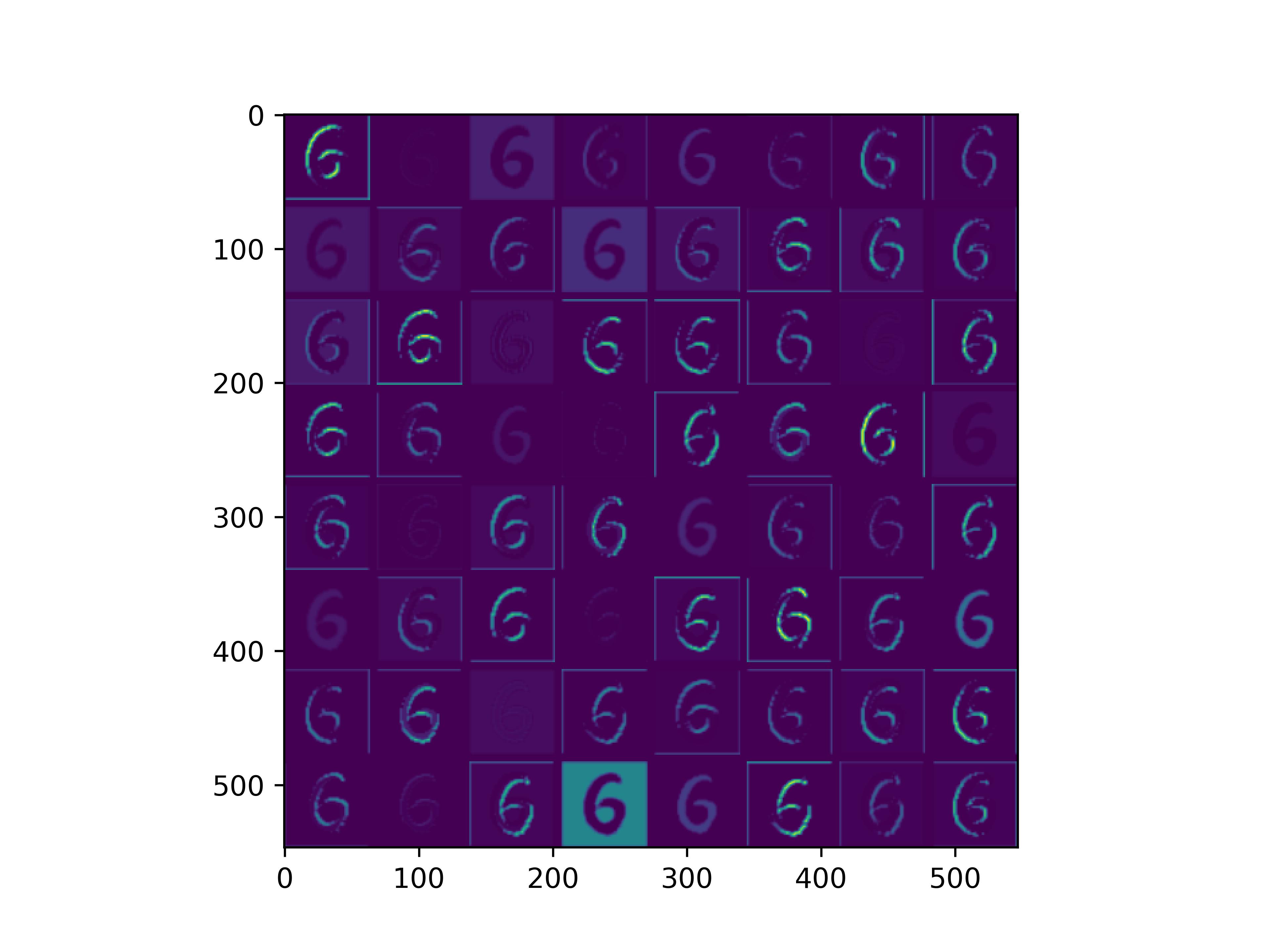
conv_block1_conv1

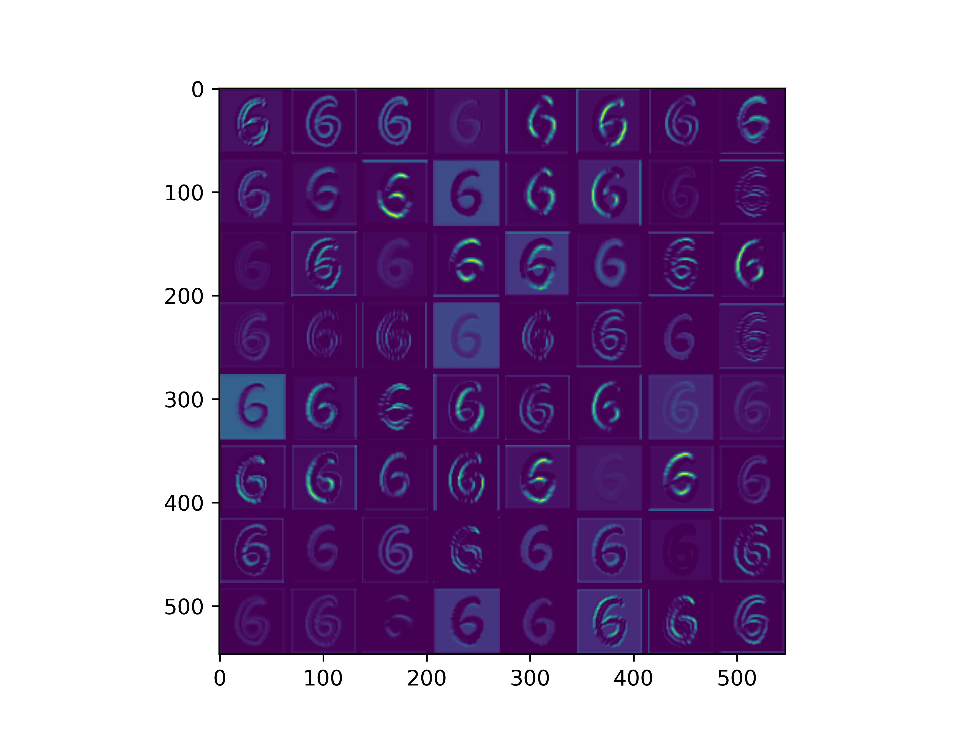
conv_block1_conv2

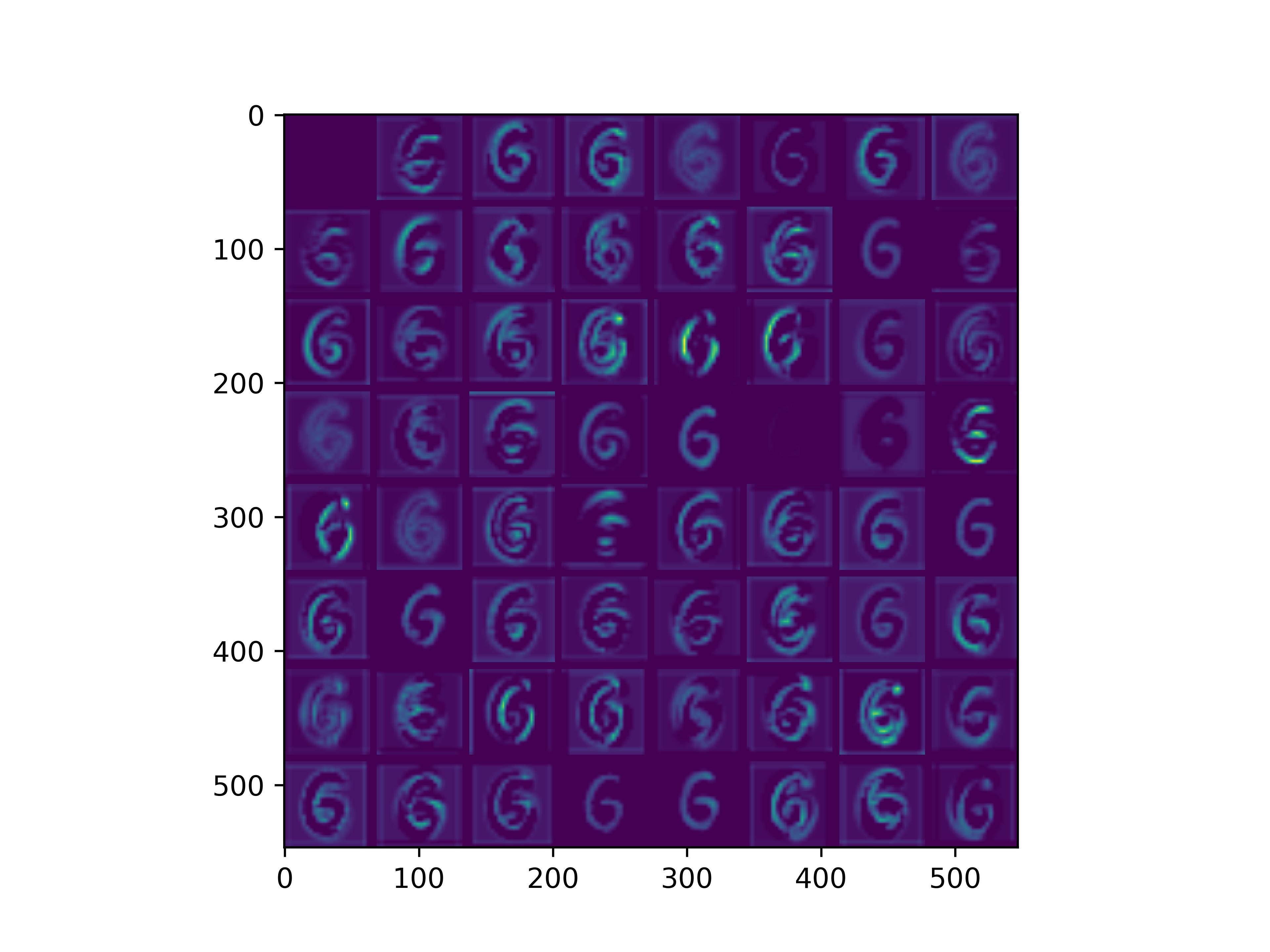
conv_block2_conv1

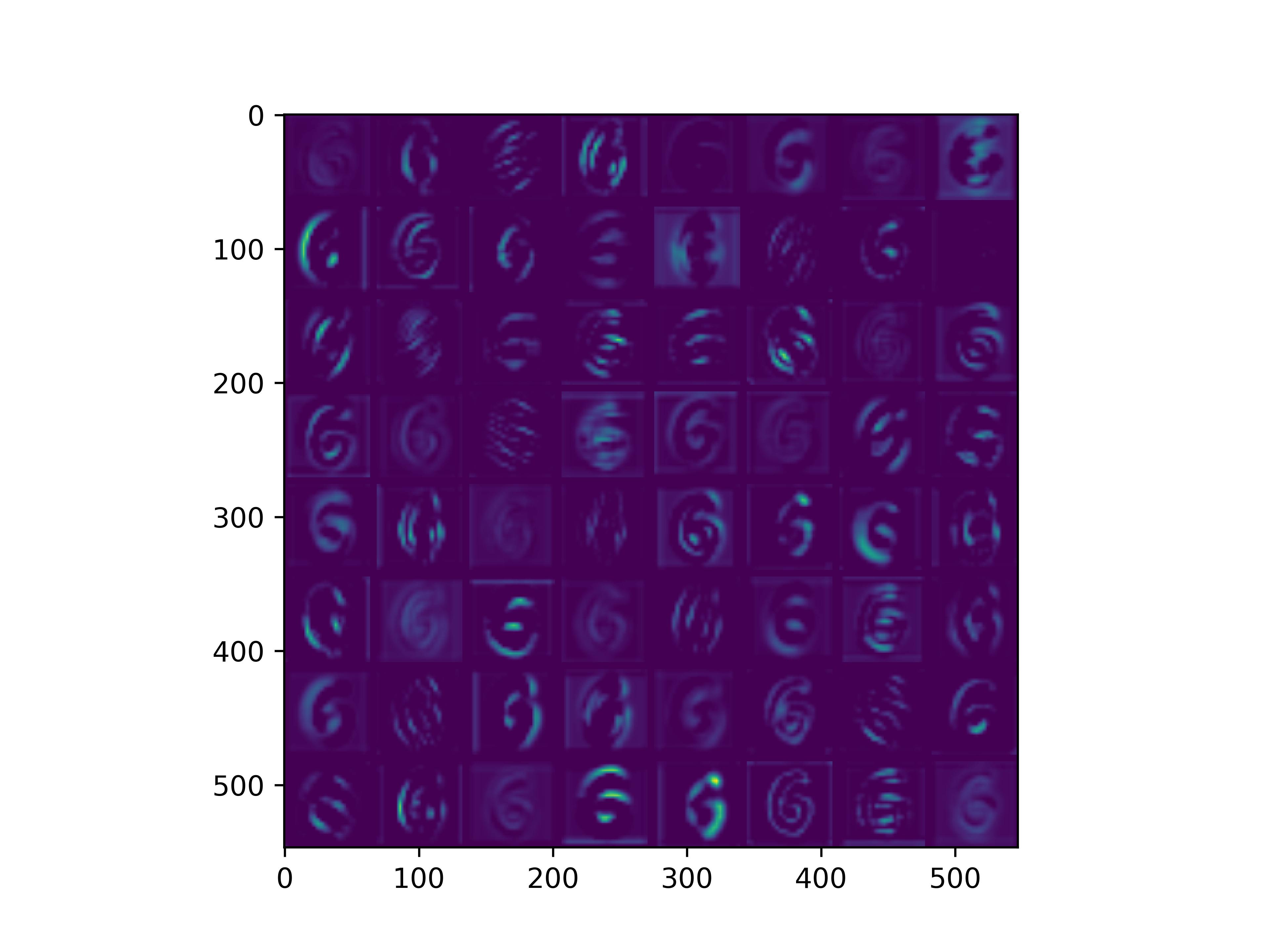
conv_block2_conv2

conv_block3_conv1

conv_block3_conv2

conv_block5_conv3

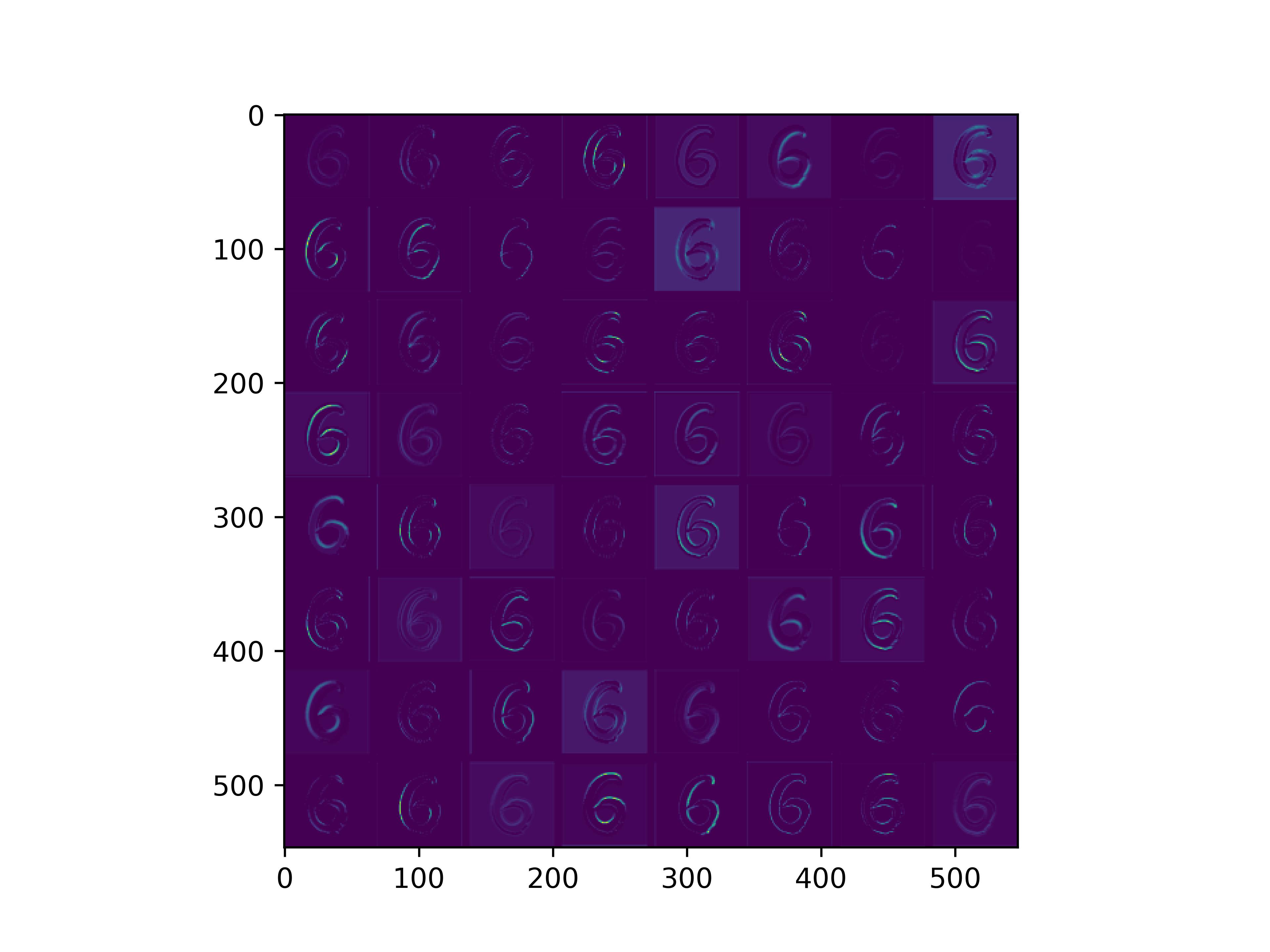
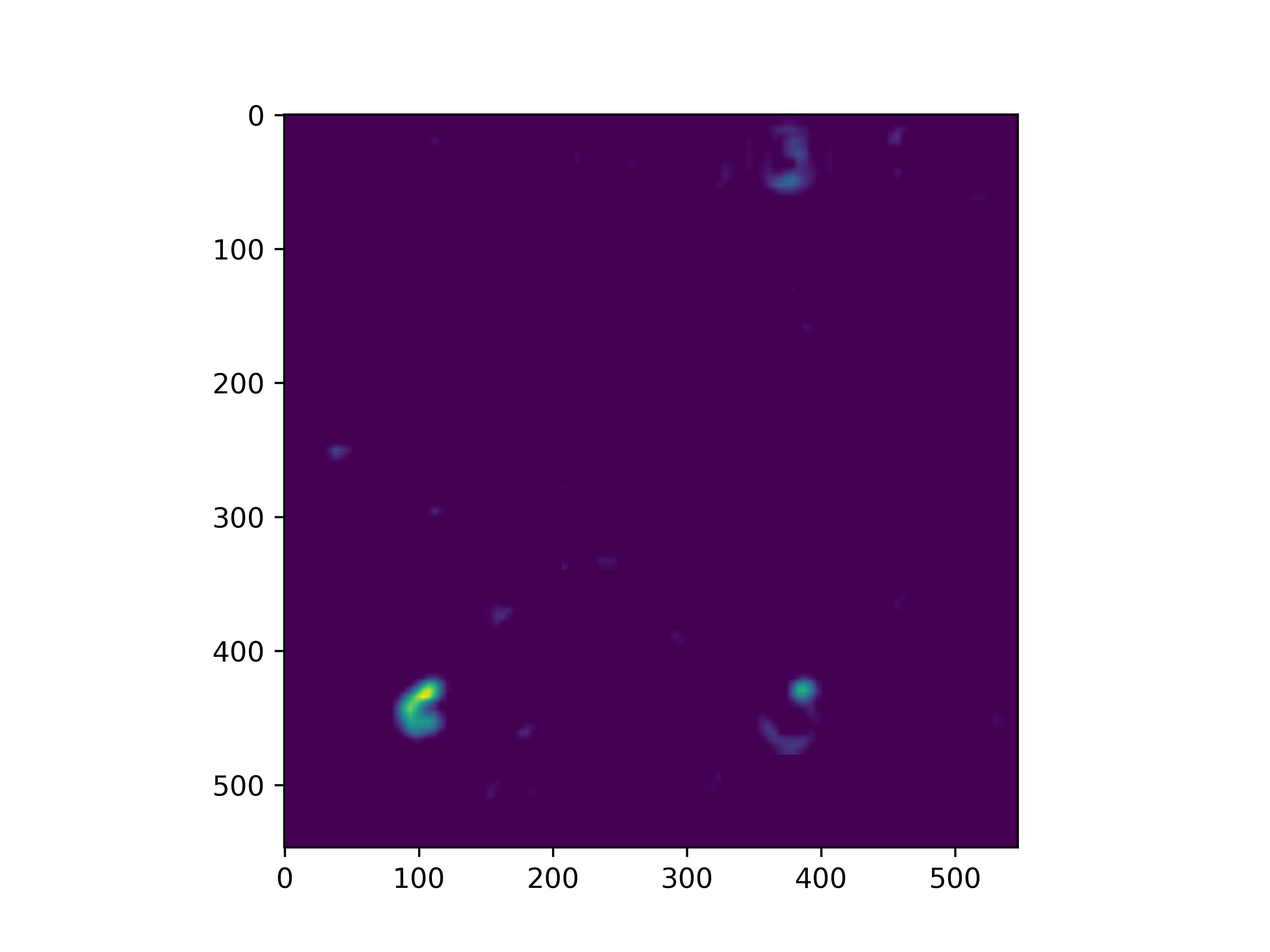
通俗来看，可以这么理解VGG16的卷积层

VGG16的卷积感知域是逐层扩大的，底层负责感知线条细节，高层负责统领综合底层的细节感知域，对目标对象进行抽象地描绘。
最底层的卷积层感知的是线条感知，最底层负责提取各种形状的数字6；越往高层，数字6的形态越来越弱，取而代之的是特定区域的激活（在上图中表现为特别明亮）程度决定了对哪些下层感知器（数字6的线条形态）予以更多的关注权重。

0x3：使用VGG16作为预训练模型，fine-tune一个手写数字识别卷积网络，再观察基模型和fine-tune模型的可视化

通过前面的章节我们知道，VGG16预训练模型不太具备手写数字识别能力，也就是说，预训练模型的样本领域和下游任务的样本领域存在较大差异。

在这种情况下，我们通过下面几个实验来更加本质地理解fine-tune在模型层面具体调整了哪些东西。

1、直接设计一个CNN卷积网络进行手写数字识别

# In -> [[Conv2D->relu]*2 -> MaxPool2D -> Dropout]*2 -> Flatten -> Dense -> Dropout -> Out
model = Sequential()

model.add(Conv2D(filters=32, kernel_size=(5, 5), padding='Same',
                 activation='relu', input_shape = (28, 28, 1)))
model.add(Conv2D(filters=32, kernel_size=(5, 5), padding='Same',
                 activation='relu'))
model.add(MaxPool2D(pool_size=(2, 2)))
model.add(Dropout(0.25))

model.add(Conv2D(filters=64, kernel_size=(3, 3), padding='Same',
                 activation='relu'))
model.add(Conv2D(filters=64, kernel_size=(3, 3), padding='Same',
                 activation='relu'))
model.add(MaxPool2D(pool_size=(2, 2), strides=(2, 2)))
model.add(Dropout(0.25))

model.add(Flatten())
model.add(Dense(256, activation="relu"))
model.add(Dropout(0.5))

上图是一个比较标准、主流的CNN卷积网络，在一个相对不大的训练集上，通过普通的设备进行训练就可以得到较好的效果。

2、冻结预训练基模型，调整下游fine-tune层参数：VGG16 without toplayer + 全连接层迁移学习

之所以选择这种模型设计结构，出于以下几点考虑：

尽量复用预训练基模型中可以迁移到下游任务的模型部分：理论上，VGG16已经基本完成了局部->整体视野的卷积核训练，这种能力在手写数字识别中也是可以复用的（存在迁移学习的前提条件），这点通过前面章节可视化卷积核的实验也可以看出。
VGG16的顶层结构设计初衷是进行1000种生活常见图形识别，并不适配10类数字识别的任务，所以toplayer需要舍弃，同时在下游接上一个新的神经网络结构，专门用于10类手写数字识别。
由于下游任何和预训练基模型存在任务领域的差异，所以下游fine-tune对训练样本集有一定的要求，因此我们需要对数据进行增强，在原数据集的基础上随机旋转、平移、缩放、产生噪音，从而更好地聚焦于数字特征的提取，而不是数据集本身。
VGG16的输入层是RGB 224*224*3彩色像素图片，MNIST手写数字是GRAY 28*28*1灰度像素图片，虽然存在一定差异，但总体上都属于像素图片领域范畴，具有一定的迁移学习的理论基础。
训练过程实际上是在训练下游fine-tune的全连接网络，前面的卷积模型参数是”固化（不可训练的）。

下面代码使用了 keras.applications.vgg16 中的 VGG16，在线获取已有的 VGG16 模型及参数，获取后冻结 VGG16 中的所有参数进行训练。

在这之后添加几层 relu 全连接以及用于多分类的 softmax 全连接，原则上基本参考了通用CNN手写数字识别卷积网络的设计。

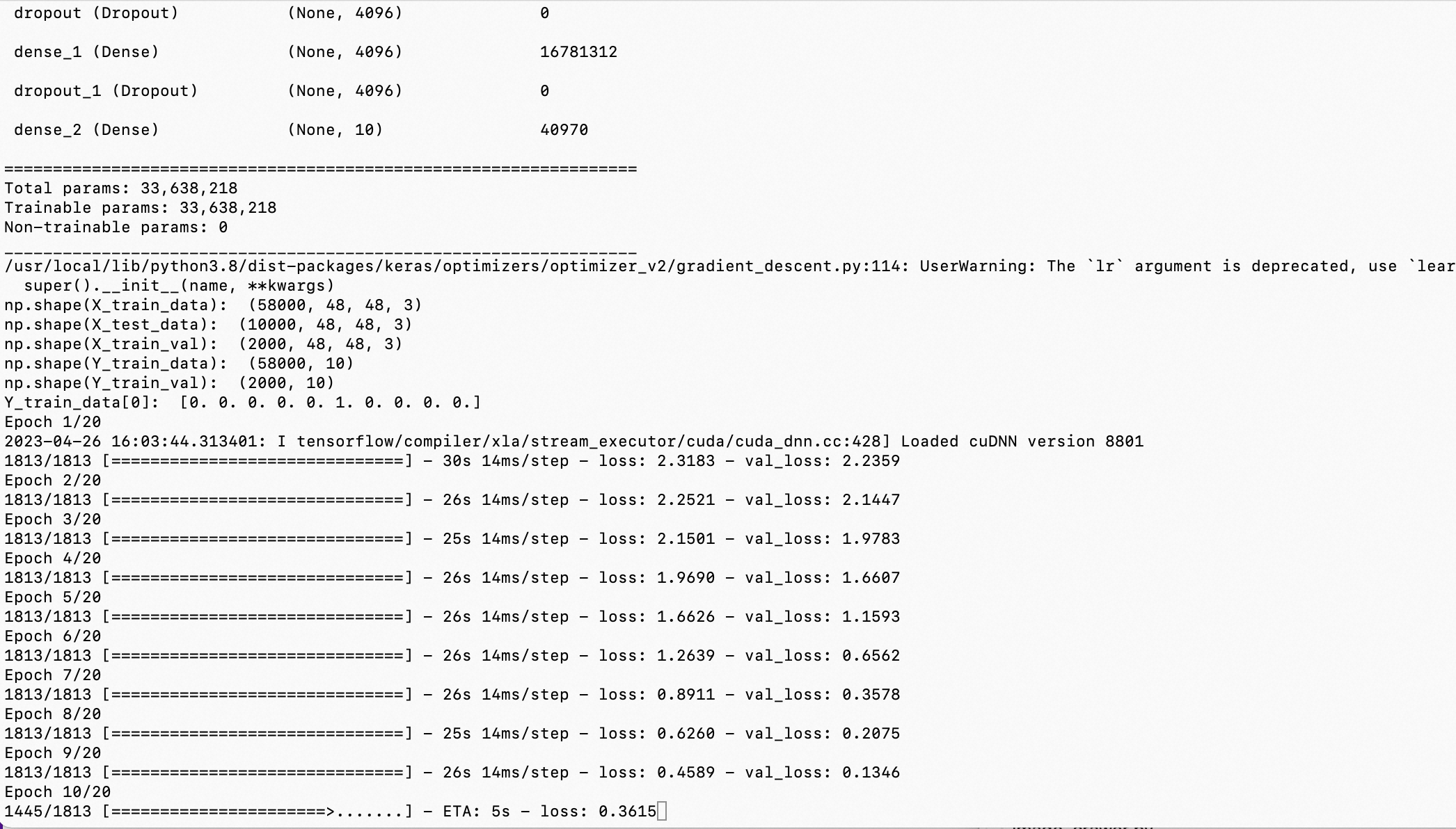
stacking之后的新的模型结构如下：

Model: "model"
_________________________________________________________________
 Layer (type)                Output Shape              Param #   
=================================================================
 input_1 (InputLayer)        [(None, 48, 48, 3)]       0         
                                                                 
 block1_conv1 (Conv2D)       (None, 48, 48, 64)        1792      
                                                                 
 block1_conv2 (Conv2D)       (None, 48, 48, 64)        36928     
                                                                 
 block1_pool (MaxPooling2D)  (None, 24, 24, 64)        0         
                                                                 
 block2_conv1 (Conv2D)       (None, 24, 24, 128)       73856     
                                                                 
 block2_conv2 (Conv2D)       (None, 24, 24, 128)       147584    
                                                                 
 block2_pool (MaxPooling2D)  (None, 12, 12, 128)       0         
                                                                 
 block3_conv1 (Conv2D)       (None, 12, 12, 256)       295168    
                                                                 
 block3_conv2 (Conv2D)       (None, 12, 12, 256)       590080    
                                                                 
 block3_conv3 (Conv2D)       (None, 12, 12, 256)       590080    
                                                                 
 block3_pool (MaxPooling2D)  (None, 6, 6, 256)         0         
                                                                 
 block4_conv1 (Conv2D)       (None, 6, 6, 512)         1180160   
                                                                 
 block4_conv2 (Conv2D)       (None, 6, 6, 512)         2359808   
                                                                 
 block4_conv3 (Conv2D)       (None, 6, 6, 512)         2359808   
                                                                 
 block4_pool (MaxPooling2D)  (None, 3, 3, 512)         0         
                                                                 
 block5_conv1 (Conv2D)       (None, 3, 3, 512)         2359808   
                                                                 
 block5_conv2 (Conv2D)       (None, 3, 3, 512)         2359808   
                                                                 
 block5_conv3 (Conv2D)       (None, 3, 3, 512)         2359808   
                                                                 
 block5_pool (MaxPooling2D)  (None, 1, 1, 512)         0         
                                                                 
 flatten (Flatten)           (None, 512)               0         
                                                                 
 dense (Dense)               (None, 4096)              2101248   
                                                                 
 dropout (Dropout)           (None, 4096)              0         
                                                                 
 dense_1 (Dense)             (None, 4096)              16781312  
                                                                 
 dropout_1 (Dropout)         (None, 4096)              0         
                                                                 
 dense_2 (Dense)             (None, 10)                40970     
                                                                 
=================================================================
Total params: 33,638,218
Trainable params: 33,638,218
Non-trainable params: 0

训练代码：

from keras.models import Model, load_model
from tensorflow.keras.applications.vgg16 import VGG16
from tensorflow.keras.preprocessing import image
from tensorflow.keras.backend import reshape, expand_dims, spatial_2d_padding, spatial_3d_padding
from tensorflow.keras.applications.vgg16 import preprocess_input, decode_predictions
from tensorflow.keras.layers import Dense, GlobalAveragePooling1D, Flatten, Dropout, Conv1D
from keras.optimizers import SGD
from keras.datasets import mnist
from keras.utils import to_categorical
import tensorflow as tf
import numpy as np
import cv2
import matplotlib.pyplot as plt

import os
os.environ["CUDA_VISIBLE_DEVICES"] = "0"


def vis_conv(images, n, name, t):
    """visualize conv output and conv filter.
    Args:
           img: original image.
           n: number of col and row.
           t: vis type.
           name: save name.
    """
    size = 64
    margin = 5

    if t == 'filter':
        results = np.zeros((n * size + 7 * margin, n * size + 7 * margin, 3))
    if t == 'conv':
        results = np.zeros((n * size + 7 * margin, n * size + 7 * margin))

    for i in range(n):
        for j in range(n):
            if t == 'filter':
                filter_img = images[i + (j * n)]
            if t == 'conv':
                filter_img = images[..., i + (j * n)]
            filter_img = cv2.resize(filter_img, (size, size))

            # Put the result in the square `(i, j)` of the results grid
            horizontal_start = i * size + i * margin
            horizontal_end = horizontal_start + size
            vertical_start = j * size + j * margin
            vertical_end = vertical_start + size
            if t == 'filter':
                results[horizontal_start: horizontal_end, vertical_start: vertical_end, :] = filter_img
            if t == 'conv':
                results[horizontal_start: horizontal_end, vertical_start: vertical_end] = filter_img

    # Display the results grid
    plt.imshow(results)
    plt.savefig('images/{}_{}.jpg'.format(t, name), dpi=600)
    plt.show()


def conv_output(model, layer_name, img):
    """Get the output of conv layer.

    Args:
           model: keras model.
           layer_name: name of layer in the model.
           img: processed input image.

    Returns:
           intermediate_output: feature map.
    """
    # this is the placeholder for the input images
    input_img = model.input

    try:
        # this is the placeholder for the conv output
        out_conv = model.get_layer(layer_name).output
    except:
        raise Exception('Not layer named {}!'.format(layer_name))

    # get the intermediate layer model
    intermediate_layer_model = Model(inputs=input_img, outputs=out_conv)

    # get the output of intermediate layer model
    intermediate_output = intermediate_layer_model.predict(img)

    return intermediate_output[0]


def get_mnist_data():
    (X_train_data, Y_train_data), (X_test_data, Y_test_data) = mnist.load_data()
    # convert Y label into one-hot
    Y_train_data = to_categorical(Y_train_data)
    Y_test_data = to_categorical(Y_test_data)
    X_train_data = X_train_data.astype('float32') / 255.0
    X_test_data = X_test_data.astype('float32') / 255.0

    # reshape the mnist data in 48*48*3
    X_train_data = expand_dims(X_train_data, axis=-1)
    X_test_data = expand_dims(X_test_data, axis=-1)
    X_train_data = tf.pad(X_train_data, [[0, 0], [2, 18], [2, 18], [1, 1]])
    X_test_data = tf.pad(X_test_data, [[0, 0], [2, 18], [2, 18], [1, 1]])

    # prepare validate/train date
    X_train_val = X_train_data[-2000:, ...]
    X_train_data = X_train_data[:-2000, ...]
    Y_train_val = Y_train_data[-2000:]
    Y_train_data = Y_train_data[:-2000]

    print("np.shape(X_train_data): ", np.shape(X_train_data))
    print("np.shape(X_test_data): ", np.shape(X_test_data))
    print("np.shape(X_train_val): ", np.shape(X_train_val))
    print("np.shape(Y_train_data): ", np.shape(Y_train_data))
    print("np.shape(Y_train_val): ", np.shape(Y_train_val))
    print("Y_train_data[0]: ", Y_train_data[0])

    return (X_train_data, Y_train_data), (X_test_data, Y_test_data), (X_train_val, Y_train_val)


def train_fine_tune():
    # create the base pre-trained model
    base_model = VGG16(weights='imagenet', include_top=False, input_shape=(48, 48, 3))

    # create a fine-tune model
    x = base_model.output
    print("base_model.input_shape: ", base_model.input_shape)
    print("base_model.input_shape[1:]: ", base_model.input_shape[1:])
    print("base_model.output_shape: ", base_model.output_shape)
    print("base_model.output_shape[1:]: ", base_model.output_shape[1:])
    # let's add a fully-connected layer
    x = Flatten()(x)
    x = Dense(4096, activation='relu')(x)
    x = Dropout(0.5)(x)
    x = Dense(4096, activation='relu')(x)
    x = Dropout(0.5)(x)
    # and a logistic layer -- let's say we have 10 classes
    predictions = Dense(10, activation='softmax')(x)

    # this is the new model(vgg16+fine-tune model) we will train
    model = Model(inputs=base_model.input, outputs=predictions)
    print("model.input_shape: ", model.input_shape)
    print("model.input_shape[1:]: ", model.input_shape[1:])
    print("model.output_shape: ", model.output_shape)
    print("model.output_shape[1:]: ", model.output_shape[1:])
    model.summary()

    # i.e. freeze all convolutional VGG16 layers
    for layer in base_model.layers:
        layer.trainable = False

    # compile the model (should be done *after* setting layers to non-trainable)
    sgd = SGD(lr=1e-5, decay=1e-6, momentum=0.5, nesterov=True)  # 优化函数，设定学习率（lr）等参数，注意，fine-tune的学习率一般要小于预训练基模型的10倍以下
    # model.compile(loss='categorical_crossentropy', optimizer="rmsprop")
    model.compile(loss='categorical_crossentropy', optimizer=sgd)

    # load the mnist data, and fine-tune the new model
    (X_train_data, Y_train_data), (X_test_data, Y_test_data), (X_train_val, Y_train_val) = get_mnist_data()

    # train the model on the new data for a few epochs
    history = model.fit(
        X_train_data, Y_train_data,
        batch_size=32,
        epochs=20,
        validation_data=(X_train_val, Y_train_val)
    )

    model.save('vgg16_plus_dnn_for_mnist.h5')


def predict():
    model = load_model("./vgg16_plus_dnn_for_mnist.h5")

    (X_train_data, Y_train_data), (X_test_data, Y_test_data), (X_train_val, Y_train_val) = get_mnist_data()

    # 查看第一张图片
    plt.imshow(X_test_data[0])
    plt.show()

    print("前十个图片对应的标签：　\n", np.argmax(Y_test_data[:10], axis=1))
    print("取前十张图片测试集预测：\n", np.argmax(model.predict(X_test_data[:10]), axis=1))   


if __name__ == '__main__':
    train_fine_tune()
    # predict()

View Code

mnist原本的图像是(，28，28)的黑白图像，但是VGG16的输入层要求的是(，224，224，)的RGB彩色图像，因此在加载mnist样本后，需要在原数据集上增加一个额外的维度，

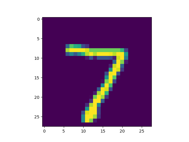
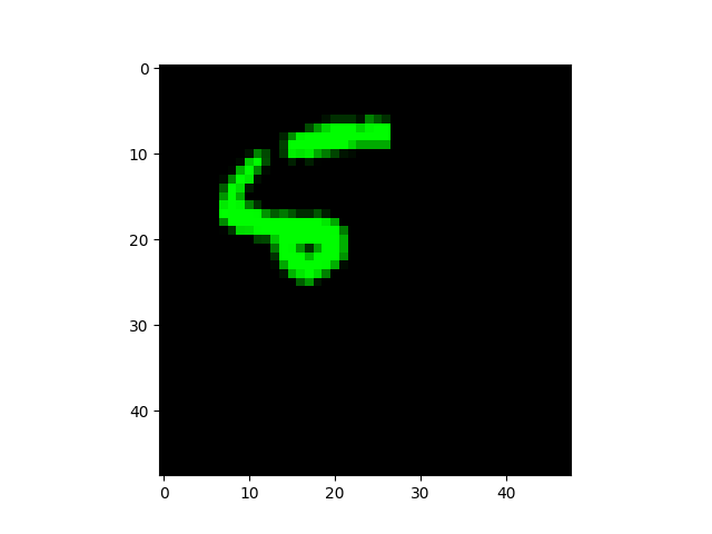
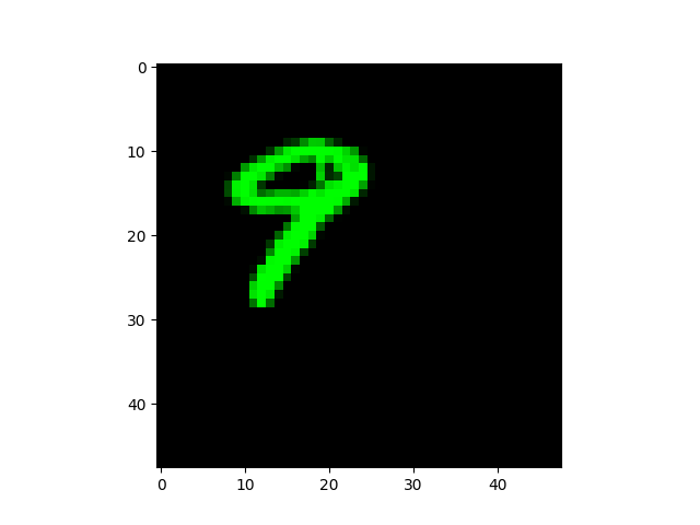
mnist数据

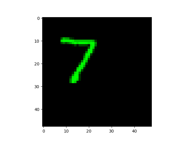
转换为适配vgg16输入层的数据格式

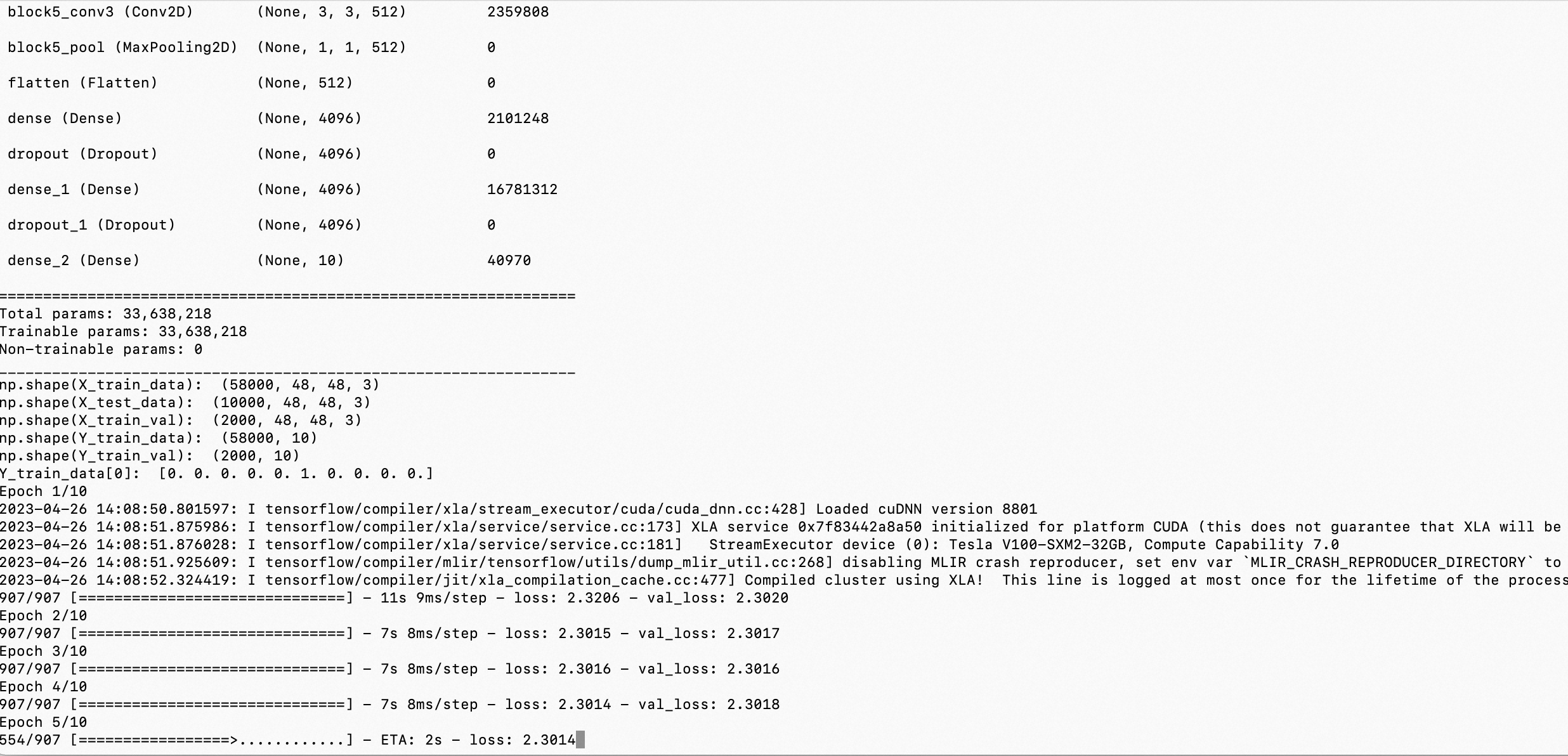
训练过程有几个点需要读者朋友注意：

从开始到最后结束，不管如何减少learning_rate、梯度更新方法、epoch数量，val_loos和loss都始终保持在2.3左右震荡而无法下降
如果参数空间本身已经找不到优化方向，则喂入再多的样本都是徒劳
预训练基模型已经的输入层相当于设定了一个数据向量化的框架，下游fine-tune的所有任务，都需要“削足适履”，将各自领域的数据都“转换”成预训练基模型要求的向量化格式。在上图中可以看到，mnist的图像在经过转换后，数字在像素矩阵中的占比变小了，同时因为多了一个像素维度层，导致整体像素的对比度都变化了

以上现象揭示了关于fine-tune的几点思考：

对于下游模型来说，如果freeze了上游基模型的参数，则上游的预训练基模型本质上可以理解为一种“先验编码器”，输入样本经过上游预训练基模型后相当于经过了一次领域经验特征工程，本身留给下游模型进行优化微调的空间就已经有限了（已经进入了相对宽域地局部最优空间中）
所谓“上游预训练基模型和下游模型领域任务的可迁移性”，在模型层面，由以下几点提现
- 预训练基模型的输入层向量化结构，决定了输入样本的向量化编码方式，即决定了特征工程
- 预训练基模型的模型结构，决定了模型所抽象描绘的非线性方程，即决定了模型所抽象的领域任务
- 预训练基模型的模型参数，代表了压缩存储了预训练样本集的知识和信息，即决定了在迁移学习时所能依据的基础知识

加载fine-tune好的模型，并对测试集进行测试，

前十个图片对应的标签：　
 [7 2 1 0 4 1 4 9 5 9]

取前十张图片测试集预测：
 [1 2 1 0 4 1 4 9 3 3]

预测错误的图片（索引：0、8、9）如下：

模型预测错误成了：1

模型预测错误成了：3

可以看到，在预训练基模型参数不变的情况下进行fine-tune，如果预训练基模型的编码方式、张量维度、张量大小等因为和下游任务不完全一样，则最终迁移学习的效果并不能达到最好。

尝试用训练好的模型，对前面的数字6进行预测，

from keras.models import Model, load_model
from tensorflow.keras.applications.vgg16 import VGG16
from tensorflow.keras.preprocessing import image
from tensorflow.keras.backend import reshape, expand_dims, spatial_2d_padding, spatial_3d_padding
from tensorflow.keras.applications.vgg16 import preprocess_input, decode_predictions
from tensorflow.keras.layers import Dense, GlobalAveragePooling1D, Flatten, Dropout, Conv1D
from keras.optimizers import SGD
from keras.datasets import mnist
from keras.utils import to_categorical
import tensorflow as tf
import numpy as np
import cv2
import matplotlib.pyplot as plt

import os
os.environ["CUDA_VISIBLE_DEVICES"] = "0"


def vis_conv(images, n, name, t):
    """visualize conv output and conv filter.
    Args:
           img: original image.
           n: number of col and row.
           t: vis type.
           name: save name.
    """
    size = 64
    margin = 5

    if t == 'filter':
        results = np.zeros((n * size + 7 * margin, n * size + 7 * margin, 3))
    if t == 'conv':
        results = np.zeros((n * size + 7 * margin, n * size + 7 * margin))

    for i in range(n):
        for j in range(n):
            if t == 'filter':
                filter_img = images[i + (j * n)]
            if t == 'conv':
                filter_img = images[..., i + (j * n)]
            filter_img = cv2.resize(filter_img, (size, size))

            # Put the result in the square `(i, j)` of the results grid
            horizontal_start = i * size + i * margin
            horizontal_end = horizontal_start + size
            vertical_start = j * size + j * margin
            vertical_end = vertical_start + size
            if t == 'filter':
                results[horizontal_start: horizontal_end, vertical_start: vertical_end, :] = filter_img
            if t == 'conv':
                results[horizontal_start: horizontal_end, vertical_start: vertical_end] = filter_img

    # Display the results grid
    plt.imshow(results)
    plt.savefig('images/{}_{}.jpg'.format(t, name), dpi=600)
    plt.show()


def conv_output(model, layer_name, img):
    """Get the output of conv layer.

    Args:
           model: keras model.
           layer_name: name of layer in the model.
           img: processed input image.

    Returns:
           intermediate_output: feature map.
    """
    # this is the placeholder for the input images
    input_img = model.input

    try:
        # this is the placeholder for the conv output
        out_conv = model.get_layer(layer_name).output
    except:
        raise Exception('Not layer named {}!'.format(layer_name))

    # get the intermediate layer model
    intermediate_layer_model = Model(inputs=input_img, outputs=out_conv)

    # get the output of intermediate layer model
    intermediate_output = intermediate_layer_model.predict(img)

    return intermediate_output[0]


def get_mnist_data():
    (X_train_data, Y_train_data), (X_test_data, Y_test_data) = mnist.load_data()
    # convert Y label into one-hot
    Y_train_data = to_categorical(Y_train_data)
    Y_test_data = to_categorical(Y_test_data)
    X_train_data = X_train_data.astype('float32') / 255.0
    X_test_data = X_test_data.astype('float32') / 255.0

    # reshape the mnist data in 48*48*3
    X_train_data = expand_dims(X_train_data, axis=-1)
    X_test_data = expand_dims(X_test_data, axis=-1)
    X_train_data = tf.pad(X_train_data, [[0, 0], [2, 18], [2, 18], [1, 1]])
    X_test_data = tf.pad(X_test_data, [[0, 0], [2, 18], [2, 18], [1, 1]])

    # prepare validate/train date
    X_train_val = X_train_data[-2000:, ...]
    X_train_data = X_train_data[:-2000, ...]
    Y_train_val = Y_train_data[-2000:]
    Y_train_data = Y_train_data[:-2000]

    print("np.shape(X_train_data): ", np.shape(X_train_data))
    print("np.shape(X_test_data): ", np.shape(X_test_data))
    print("np.shape(X_train_val): ", np.shape(X_train_val))
    print("np.shape(Y_train_data): ", np.shape(Y_train_data))
    print("np.shape(Y_train_val): ", np.shape(Y_train_val))
    print("Y_train_data[0]: ", Y_train_data[0])

    return (X_train_data, Y_train_data), (X_test_data, Y_test_data), (X_train_val, Y_train_val)


def train_fine_tune(base_model_freeze=True):
    # create the base pre-trained model
    base_model = VGG16(weights='imagenet', include_top=False, input_shape=(48, 48, 3))

    # create a fine-tune model
    x = base_model.output
    print("base_model.input_shape: ", base_model.input_shape)
    print("base_model.input_shape[1:]: ", base_model.input_shape[1:])
    print("base_model.output_shape: ", base_model.output_shape)
    print("base_model.output_shape[1:]: ", base_model.output_shape[1:])
    # let's add a fully-connected layer
    x = Flatten()(x)
    x = Dense(4096, activation='relu')(x)
    x = Dropout(0.5)(x)
    x = Dense(4096, activation='relu')(x)
    x = Dropout(0.5)(x)
    # and a logistic layer -- let's say we have 10 classes
    predictions = Dense(10, activation='softmax')(x)

    # this is the new model(vgg16+fine-tune model) we will train
    model = Model(inputs=base_model.input, outputs=predictions)
    print("model.input_shape: ", model.input_shape)
    print("model.input_shape[1:]: ", model.input_shape[1:])
    print("model.output_shape: ", model.output_shape)
    print("model.output_shape[1:]: ", model.output_shape[1:])
    model.summary()

    if base_model_freeze:
        # i.e. freeze all convolutional VGG16 layers
        for layer in base_model.layers:
            layer.trainable = False
    else:
        for layer in base_model.layers:
            layer.trainable = True

    # compile the model (should be done *after* setting layers to non-trainable)
    sgd = SGD(lr=1e-5, decay=1e-6, momentum=0.5, nesterov=True)  # 优化函数，设定学习率（lr）等参数，注意，fine-tune的学习率一般要小于预训练基模型的10倍以下
    # model.compile(loss='categorical_crossentropy', optimizer="rmsprop")
    model.compile(loss='categorical_crossentropy', optimizer=sgd)

    # load the mnist data, and fine-tune the new model
    (X_train_data, Y_train_data), (X_test_data, Y_test_data), (X_train_val, Y_train_val) = get_mnist_data()

    # train the model on the new data for a few epochs
    history = model.fit(
        X_train_data, Y_train_data,
        batch_size=32,
        epochs=20,
        validation_data=(X_train_val, Y_train_val)
    )

    if base_model_freeze:
        model.save('vgg16_plus_dnn_for_mnist_base_model_freeze.h5')
    else:
        model.save('vgg16_plus_dnn_for_mnist_base_model_train.h5')


def predict(base_model_freeze=True):
    if base_model_freeze:
        model = load_model("./vgg16_plus_dnn_for_mnist_base_model_freeze.h5")
    else:
        model = load_model("./vgg16_plus_dnn_for_mnist_base_model_train.h5")

    (X_train_data, Y_train_data), (X_test_data, Y_test_data), (X_train_val, Y_train_val) = get_mnist_data()

    # 查看图片
    plt.imshow(X_test_data[0])
    plt.show()
    #plt.imshow(X_test_data[8])
    #plt.show()
    #plt.imshow(X_test_data[9])
    #plt.show()

    print("前十个图片对应的标签：　\n", np.argmax(Y_test_data[:10], axis=1))
    print("取前十张图片测试集预测：\n", np.argmax(model.predict(X_test_data[:10]), axis=1))


def visual_cnnkernel_with_number_6(base_model_freeze=True):
    if base_model_freeze:
        model = load_model("./vgg16_plus_dnn_for_mnist_base_model_freeze.h5")
    else:
        model = load_model("./vgg16_plus_dnn_for_mnist_base_model_train.h5")

    img_path = '6.webp'
    img = image.load_img(img_path, target_size=(48, 48))
    plt.imshow(img)
    plt.show()

    x = image.img_to_array(img)
    x = np.expand_dims(x, axis=0)
    x = preprocess_input(x)
    print("np.shape(x): ", np.shape(x))

    preds = model.predict(x)
    # decode the results into a list of tuples (class, description, probability)
    # (one such list for each sample in the batch)
    print('Predicted:', np.argmax(preds, axis=1))

    conv_output_block1_conv1 = conv_output(model, "block1_conv1", x)
    print("block1_conv1: ", conv_output_block1_conv1)
    vis_conv(conv_output_block1_conv1, 8, "block1_conv1", 'conv')

    conv_output_block1_conv2 = conv_output(model, "block1_conv2", x)
    print("block1_conv2: ", conv_output_block1_conv2)
    vis_conv(conv_output_block1_conv2, 8, "block1_conv2", 'conv')

    conv_output_block2_conv1 = conv_output(model, "block2_conv1", x)
    print("block2_conv1: ", conv_output_block2_conv1)
    vis_conv(conv_output_block2_conv1, 8, "block2_conv1", 'conv')

    conv_output_block2_conv2 = conv_output(model, "block2_conv2", x)
    print("block2_conv2: ", conv_output_block2_conv2)
    vis_conv(conv_output_block2_conv2, 8, "block2_conv2", 'conv')

    conv_output_block3_conv1 = conv_output(model, "block3_conv1", x)
    print("block3_conv1: ", conv_output_block3_conv1)
    vis_conv(conv_output_block3_conv1, 8, "block3_conv1", 'conv')

    conv_output_block3_conv2 = conv_output(model, "block3_conv2", x)
    print("block3_conv2: ", conv_output_block3_conv2)
    vis_conv(conv_output_block3_conv2, 8, "block3_conv2", 'conv')

    conv_output_block5_conv3 = conv_output(model, "block5_conv3", x)
    print("block5_conv3: ", conv_output_block5_conv3)
    vis_conv(conv_output_block5_conv3, 8, "block5_conv3", 'conv')

    print("fc1: ", conv_output(model, "fc1", x))
    print("fc2: ", conv_output(model, "fc2", x))
    print("predictions: ", conv_output(model, "predictions", x))


def vgg16_predict():
    model = VGG16(weights='imagenet')

    img_6_path = '6.webp'
    img_elephant_path = 'elephant.png'
    img = image.load_img(img_elephant_path, target_size=(224, 224))
    x = image.img_to_array(img)
    x = np.expand_dims(x, axis=0)
    x = preprocess_input(x)

    preds = model.predict(x)
    # decode the results into a list of tuples (class, description, probability)
    # (one such list for each sample in the batch)
    print('Predicted:', decode_predictions(preds, top=3)[0])


if __name__ == '__main__':
    # train_fine_tune(base_model_freeze=True)
    # predict(base_model_freeze=False)
    visual_cnnkernel_with_number_6(base_model_freeze=True)
    # vgg16_predict()

View Code

预测结果为：

Predicted: [0]

3、允许预训练基模型参数微调，同时调整下游fine-tune层参数：VGG16 without toplayer + 全连接层迁移学习

现在我们调整一下策略：

VGG16预训练基模型虽然也是卷积神经网络，训练过程也充分拟合了，但是训练样本库并不包含手写数字图片，因此可以推断VGG16并不包含手写数字识别的“知识”
基于VGG16+fine-tune进行手写数字识别，本质上是一个迁移学习，因此基模型本身也需要进行一定的学习调整

from keras.models import Model, load_model
from tensorflow.keras.applications.vgg16 import VGG16
from tensorflow.keras.preprocessing import image
from tensorflow.keras.backend import reshape, expand_dims, spatial_2d_padding, spatial_3d_padding
from tensorflow.keras.applications.vgg16 import preprocess_input, decode_predictions
from tensorflow.keras.layers import Dense, GlobalAveragePooling1D, Flatten, Dropout, Conv1D
from keras.optimizers import SGD
from keras.datasets import mnist
from keras.utils import to_categorical
import tensorflow as tf
import numpy as np
import cv2
import matplotlib.pyplot as plt

import os
os.environ["CUDA_VISIBLE_DEVICES"] = "0"


def vis_conv(images, n, name, t):
    """visualize conv output and conv filter.
    Args:
           img: original image.
           n: number of col and row.
           t: vis type.
           name: save name.
    """
    size = 64
    margin = 5

    if t == 'filter':
        results = np.zeros((n * size + 7 * margin, n * size + 7 * margin, 3))
    if t == 'conv':
        results = np.zeros((n * size + 7 * margin, n * size + 7 * margin))

    for i in range(n):
        for j in range(n):
            if t == 'filter':
                filter_img = images[i + (j * n)]
            if t == 'conv':
                filter_img = images[..., i + (j * n)]
            filter_img = cv2.resize(filter_img, (size, size))

            # Put the result in the square `(i, j)` of the results grid
            horizontal_start = i * size + i * margin
            horizontal_end = horizontal_start + size
            vertical_start = j * size + j * margin
            vertical_end = vertical_start + size
            if t == 'filter':
                results[horizontal_start: horizontal_end, vertical_start: vertical_end, :] = filter_img
            if t == 'conv':
                results[horizontal_start: horizontal_end, vertical_start: vertical_end] = filter_img

    # Display the results grid
    plt.imshow(results)
    plt.savefig('images/{}_{}.jpg'.format(t, name), dpi=600)
    plt.show()


def conv_output(model, layer_name, img):
    """Get the output of conv layer.

    Args:
           model: keras model.
           layer_name: name of layer in the model.
           img: processed input image.

    Returns:
           intermediate_output: feature map.
    """
    # this is the placeholder for the input images
    input_img = model.input

    try:
        # this is the placeholder for the conv output
        out_conv = model.get_layer(layer_name).output
    except:
        raise Exception('Not layer named {}!'.format(layer_name))

    # get the intermediate layer model
    intermediate_layer_model = Model(inputs=input_img, outputs=out_conv)

    # get the output of intermediate layer model
    intermediate_output = intermediate_layer_model.predict(img)

    return intermediate_output[0]


def get_mnist_data():
    (X_train_data, Y_train_data), (X_test_data, Y_test_data) = mnist.load_data()
    # convert Y label into one-hot
    Y_train_data = to_categorical(Y_train_data)
    Y_test_data = to_categorical(Y_test_data)
    X_train_data = X_train_data.astype('float32') / 255.0
    X_test_data = X_test_data.astype('float32') / 255.0

    # reshape the mnist data in 48*48*3
    X_train_data = expand_dims(X_train_data, axis=-1)
    X_test_data = expand_dims(X_test_data, axis=-1)
    X_train_data = tf.pad(X_train_data, [[0, 0], [2, 18], [2, 18], [1, 1]])
    X_test_data = tf.pad(X_test_data, [[0, 0], [2, 18], [2, 18], [1, 1]])

    # prepare validate/train date
    X_train_val = X_train_data[-2000:, ...]
    X_train_data = X_train_data[:-2000, ...]
    Y_train_val = Y_train_data[-2000:]
    Y_train_data = Y_train_data[:-2000]

    print("np.shape(X_train_data): ", np.shape(X_train_data))
    print("np.shape(X_test_data): ", np.shape(X_test_data))
    print("np.shape(X_train_val): ", np.shape(X_train_val))
    print("np.shape(Y_train_data): ", np.shape(Y_train_data))
    print("np.shape(Y_train_val): ", np.shape(Y_train_val))
    print("Y_train_data[0]: ", Y_train_data[0])

    return (X_train_data, Y_train_data), (X_test_data, Y_test_data), (X_train_val, Y_train_val)


def train_fine_tune(base_model_freeze=True):
    # create the base pre-trained model
    base_model = VGG16(weights='imagenet', include_top=False, input_shape=(48, 48, 3))

    # create a fine-tune model
    x = base_model.output
    print("base_model.input_shape: ", base_model.input_shape)
    print("base_model.input_shape[1:]: ", base_model.input_shape[1:])
    print("base_model.output_shape: ", base_model.output_shape)
    print("base_model.output_shape[1:]: ", base_model.output_shape[1:])
    # let's add a fully-connected layer
    x = Flatten()(x)
    x = Dense(4096, activation='relu')(x)
    x = Dropout(0.5)(x)
    x = Dense(4096, activation='relu')(x)
    x = Dropout(0.5)(x)
    # and a logistic layer -- let's say we have 10 classes
    predictions = Dense(10, activation='softmax')(x)

    # this is the new model(vgg16+fine-tune model) we will train
    model = Model(inputs=base_model.input, outputs=predictions)
    print("model.input_shape: ", model.input_shape)
    print("model.input_shape[1:]: ", model.input_shape[1:])
    print("model.output_shape: ", model.output_shape)
    print("model.output_shape[1:]: ", model.output_shape[1:])
    model.summary()

    if base_model_freeze:
        # i.e. freeze all convolutional VGG16 layers
        for layer in base_model.layers:
            layer.trainable = False
    else:
        for layer in base_model.layers:
            layer.trainable = True

    # compile the model (should be done *after* setting layers to non-trainable)
    sgd = SGD(lr=1e-5, decay=1e-6, momentum=0.5, nesterov=True)  # 优化函数，设定学习率（lr）等参数，注意，fine-tune的学习率一般要小于预训练基模型的10倍以下
    # model.compile(loss='categorical_crossentropy', optimizer="rmsprop")
    model.compile(loss='categorical_crossentropy', optimizer=sgd)

    # load the mnist data, and fine-tune the new model
    (X_train_data, Y_train_data), (X_test_data, Y_test_data), (X_train_val, Y_train_val) = get_mnist_data()

    # train the model on the new data for a few epochs
    history = model.fit(
        X_train_data, Y_train_data,
        batch_size=32,
        epochs=20,
        validation_data=(X_train_val, Y_train_val)
    )

    if base_model_freeze:
        model.save('vgg16_plus_dnn_for_mnist_base_model_freeze.h5')
    else:
        model.save('vgg16_plus_dnn_for_mnist_base_model_train.h5')


def predict():
    model = load_model("./vgg16_plus_dnn_for_mnist.h5")

    (X_train_data, Y_train_data), (X_test_data, Y_test_data), (X_train_val, Y_train_val) = get_mnist_data()

    # 查看图片
    plt.imshow(X_test_data[0])
    plt.show()
    plt.imshow(X_test_data[8])
    plt.show()
    plt.imshow(X_test_data[9])
    plt.show()

    print("前十个图片对应的标签：　\n", np.argmax(Y_test_data[:10], axis=1))
    print("取前十张图片测试集预测：\n", np.argmax(model.predict(X_test_data[:10]), axis=1))


def visual_cnnkernel_with_number_6():
    img_path = '6.webp'
    img = image.load_img(img_path, target_size=(224, 224))
    plt.imshow(img)
    plt.show()

    x = image.img_to_array(img)
    x = np.expand_dims(x, axis=0)
    x = preprocess_input(x)
    print("np.shape(x): ", np.shape(x))


if __name__ == '__main__':
    train_fine_tune(base_model_freeze=False)
    # predict()
    # visual_cnnkernel_with_number_6()

View Code

训练过程有几个点需要读者朋友注意：

相比freeze预训练基模型，允许预训练基模型参数微调后，训练过程的val_loss和loss都开始了稳步下降，这说明了预训练基模型+fine-tune模型整体都在不断朝着拟合手写数字图像特征的方向优化。反过来讲，读者可以注意上之前的章节中freeze了基模型的参数，val_loss和loss始终下不来，模型呈现出了一种欠拟合的状态。
预训练基模型自身并不具备手写数字识别的知识，自身也需要针对手写数字识别这个下游场景进行再学习和微调。

加载fine-tune好的模型，并对测试集进行测试，

前十个图片对应的标签：　
 [7 2 1 0 4 1 4 9 5 9]

取前十张图片测试集预测：
 [7 2 1 0 4 1 4 9 5 9]

可以看到，允许了预训练基模型的参数调整后，在mnist数据集上进行fine-tune，得到的最终模型，很好地适配了新的识别任务。

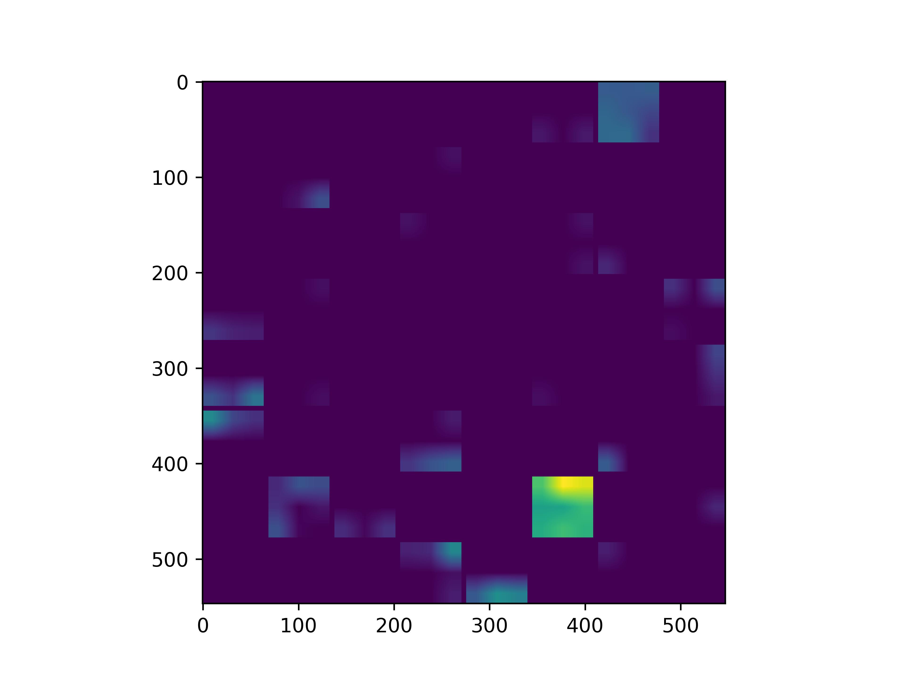
可视化基模型卷积核，观察基模型卷积核在fine-tune前后的变化。

conv_block1_conv1

conv_block1_conv2

conv_block2_conv1

conv_block2_conv2

conv_block3_conv1

conv_block3_conv2

conv_block5_conv3

可以看到，经过fine-tune之后，基模型的卷积核的感知野和感知强度变大了，这也是为什么fine-tune之后识别mnist手写数字识别能力变强的原因。

尝试用训练好的模型，对前面的数字6进行预测，

Predicted: [0]

可以看到，

不管是否freeze预训练基模型参数，用于fine-tune的数据集对最终模型的预测能力起到了很重要的作用，对于超出训练集的样本，不管是freeze基模型还是允许基模型参数调整，最终fine-tune出的模型，都无法很好地适配在训练阶段从未见过的新样本

0x4：用于下游任务的样本量大小对fine-tune效果的影响

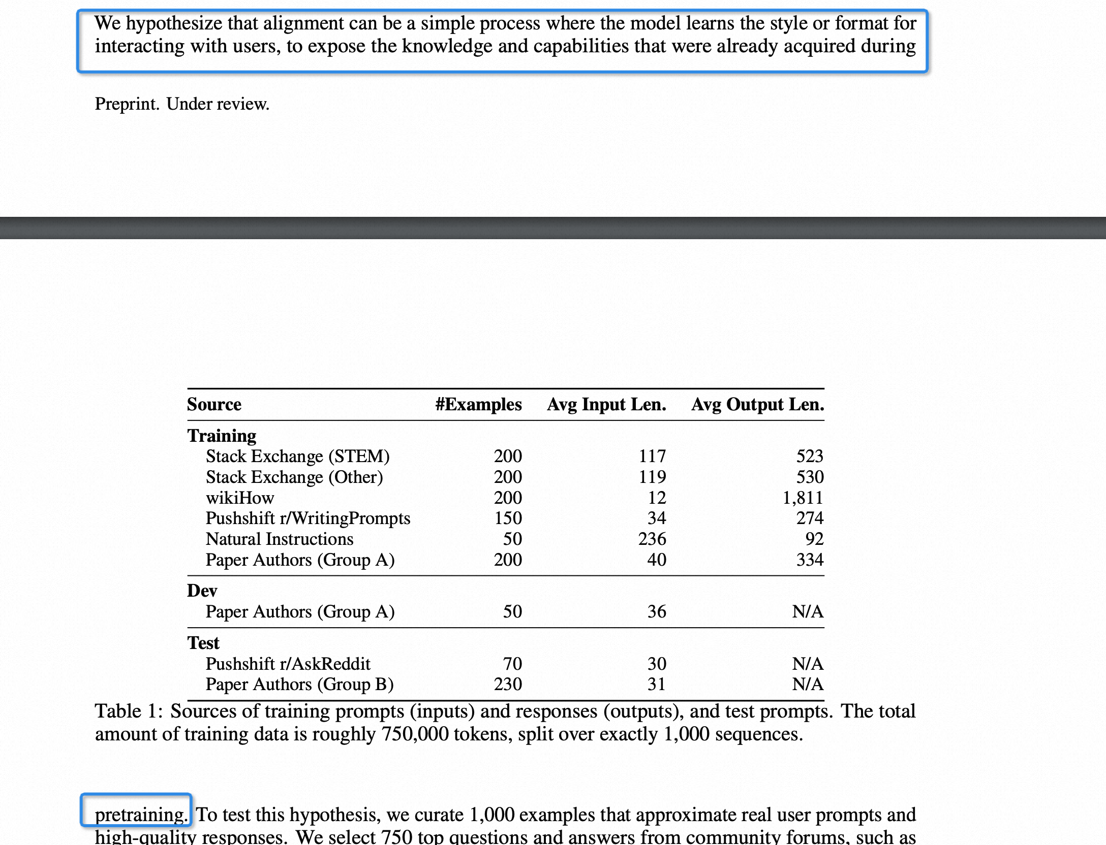
这篇论文提出了一个假设：指令微调只是让模型学会这种风格，引出这些知识，其实这些能力在预训练就已经预备了

Meta最新650亿参数模型LIMA，仅用1000个样本，实现与GPT-4相匹敌的性能。

论文中，研究人员将这一突破称为「表面对齐假设」（Superficial Alignment Hypothesis）。实验证明了，大语言模型在预训练阶段就已习得大部分知识，仅用有限的指令微调数据，足以教会模型产生高质量的内容。

它表明，所谓预训练后的对齐阶段，主要是让模型学会一种特定的风格或格式，这种风格或格式在与用户交互时可以被模型回忆起来。因此，「微调」更多是关于风格，而不是实质。

LIMA的结果表明，实际上，利用简单的方法就可以解决对齐和微调AI模型这类复杂问题。这与诸如OpenAI的RLHF那些，特别繁琐和复杂的微调过程，形成了鲜明的对比。

团队通过消融实验，研究了训练数据多样性、质量和数量的影响。

Meta发现，为了对齐目的，提高输入多样性和输出质量有可测量的正面效应，而单独增加数量却没有。

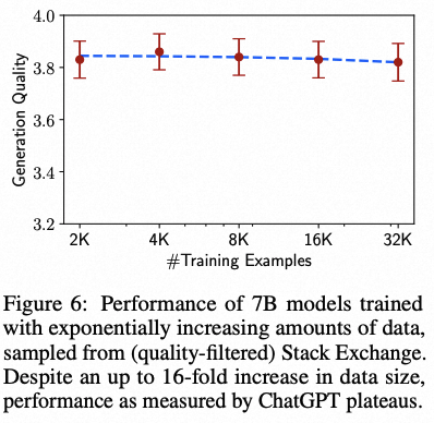
如此一来也暗示了，对齐的规模法则不必然只受数量影响，而更可能是在保持高质量响应的同时，提升提示的多样性。

我们的实验背景是VGG16基模型（允许基模型参数调整）+下游stackDNN模型，通过输入MNIST手写图片（默认都是高质量样本），尝试实现从VGG16原本的图像识别向手写数字识别这个新的end task迁移。

在整个实验中，控制和调整的变量包括：

样本量
epochs训练轮次
学习率
batchsize

观察下列两个指标：

fine-tune收敛性能（acc、loss）
fine-tune后模型泛化性能（test集预测）

代码如下：

from keras.models import Model, load_model
from tensorflow.keras.applications.vgg16 import VGG16
from tensorflow.keras.preprocessing import image
from tensorflow.keras.backend import reshape, expand_dims, spatial_2d_padding, spatial_3d_padding, arange, concatenate
from tensorflow.keras.applications.vgg16 import preprocess_input, decode_predictions
from tensorflow.keras.layers import Dense, GlobalAveragePooling1D, Flatten, Dropout, Conv1D
from keras.optimizers import SGD
from keras.datasets import mnist
from keras.utils import to_categorical
import tensorflow as tf
import numpy as np
import cv2
import matplotlib.pyplot as plt
import printfile as pf

import os
os.environ["CUDA_VISIBLE_DEVICES"] = "0"


def vis_conv(images, n, name, t):
    """visualize conv output and conv filter.
    Args:
           img: original image.
           n: number of col and row.
           t: vis type.
           name: save name.
    """
    size = 64
    margin = 5

    if t == 'filter':
        results = np.zeros((n * size + 7 * margin, n * size + 7 * margin, 3))
    if t == 'conv':
        results = np.zeros((n * size + 7 * margin, n * size + 7 * margin))

    for i in range(n):
        for j in range(n):
            if t == 'filter':
                filter_img = images[i + (j * n)]
            if t == 'conv':
                filter_img = images[..., i + (j * n)]
            filter_img = cv2.resize(filter_img, (size, size))

            # Put the result in the square `(i, j)` of the results grid
            horizontal_start = i * size + i * margin
            horizontal_end = horizontal_start + size
            vertical_start = j * size + j * margin
            vertical_end = vertical_start + size
            if t == 'filter':
                results[horizontal_start: horizontal_end, vertical_start: vertical_end, :] = filter_img
            if t == 'conv':
                results[horizontal_start: horizontal_end, vertical_start: vertical_end] = filter_img

    # Display the results grid
    plt.imshow(results)
    plt.savefig('images/{}_{}.jpg'.format(t, name), dpi=600)
    plt.show()


def conv_output(model, layer_name, img):
    """Get the output of conv layer.

    Args:
           model: keras model.
           layer_name: name of layer in the model.
           img: processed input image.

    Returns:
           intermediate_output: feature map.
    """
    # this is the placeholder for the input images
    input_img = model.input

    try:
        # this is the placeholder for the conv output
        out_conv = model.get_layer(layer_name).output
    except:
        raise Exception('Not layer named {}!'.format(layer_name))

    # get the intermediate layer model
    intermediate_layer_model = Model(inputs=input_img, outputs=out_conv)

    # get the output of intermediate layer model
    intermediate_output = intermediate_layer_model.predict(img)

    return intermediate_output[0]


def get_mnist_data(cuoff_rate=1, img_dim=48):
    (X_train_data, Y_train_data), (X_test_data, Y_test_data) = mnist.load_data()
    # convert Y label into one-hot
    Y_train_data = to_categorical(Y_train_data)
    Y_test_data = to_categorical(Y_test_data)

    # cutoff by cuoff_rate
    Y_train_data = Y_train_data[:int(np.shape(Y_train_data)[0] * cuoff_rate)]
    Y_test_data = Y_test_data[:int(np.shape(Y_test_data)[0] * cuoff_rate)]
    X_train_data = X_train_data[:int(np.shape(X_train_data)[0] * cuoff_rate), ...]
    X_test_data = X_test_data[:int(np.shape(X_test_data)[0] * cuoff_rate), ...]

    # expand the dim into 1000
    # Y_train_data = concatenate((Y_train_data, np.zeros((np.shape(Y_train_data)[0], 990))), axis=1)
    # Y_test_data = concatenate((Y_test_data, np.zeros((np.shape(Y_test_data)[0], 990))), axis=1)
    # normalize
    X_train_data = X_train_data.astype('float32') / 255.0
    X_test_data = X_test_data.astype('float32') / 255.0

    # reshape the mnist data in 224*224*3
    X_train_data = expand_dims(X_train_data, axis=-1)
    X_test_data = expand_dims(X_test_data, axis=-1)
    X_train_data = tf.pad(X_train_data, [[0, 0], [2, (img_dim-30)], [2, (img_dim-30)], [1, 1]])
    X_test_data = tf.pad(X_test_data, [[0, 0], [2, (img_dim-30)], [2, (img_dim-30)], [1, 1]])

    # prepare validate/train date
    X_train_val = X_train_data[-int(np.shape(X_train_data)[0] * 0.2):, ...]
    X_train_data = X_train_data[:-int(np.shape(X_train_data)[0] * 0.2), ...]
    Y_train_val = Y_train_data[-int(np.shape(Y_train_data)[0] * 0.2):]
    Y_train_data = Y_train_data[:-int(np.shape(Y_train_data)[0] * 0.2)]

    print("np.shape(X_train_data): ", np.shape(X_train_data))
    print("np.shape(X_test_data): ", np.shape(X_test_data))
    print("np.shape(X_train_val): ", np.shape(X_train_val))
    print("np.shape(Y_train_data): ", np.shape(Y_train_data))
    print("np.shape(Y_train_val): ", np.shape(Y_train_val))
    print("Y_train_data[0]: ", Y_train_data[0])

    return (X_train_data, Y_train_data), (X_test_data, Y_test_data), (X_train_val, Y_train_val)


def train_fine_tune(base_model_freeze=True):
    # create the base pre-trained model
    base_model = VGG16(weights='imagenet', include_top=False, input_shape=(48, 48, 3))

    # create a fine-tune model
    x = base_model.output
    print("base_model.input_shape: ", base_model.input_shape)
    print("base_model.input_shape[1:]: ", base_model.input_shape[1:])
    print("base_model.output_shape: ", base_model.output_shape)
    print("base_model.output_shape[1:]: ", base_model.output_shape[1:])
    # let's add a fully-connected layer
    x = Flatten()(x)
    x = Dense(4096, activation='relu')(x)
    x = Dropout(0.5)(x)
    x = Dense(4096, activation='relu')(x)
    x = Dropout(0.5)(x)
    # and a logistic layer -- let's say we have 10 classes
    predictions = Dense(10, activation='softmax')(x)

    # this is the new model(vgg16+fine-tune model) we will train
    model = Model(inputs=base_model.input, outputs=predictions)
    print("model.input_shape: ", model.input_shape)
    print("model.input_shape[1:]: ", model.input_shape[1:])
    print("model.output_shape: ", model.output_shape)
    print("model.output_shape[1:]: ", model.output_shape[1:])
    model.summary()

    if base_model_freeze:
        # i.e. freeze all convolutional VGG16 layers
        for layer in base_model.layers:
            layer.trainable = False
    else:
        for layer in base_model.layers:
            layer.trainable = True

    # compile the model (should be done *after* setting layers to non-trainable)
    sgd = SGD(lr=1e-5, decay=1e-6, momentum=0.5, nesterov=True)  # 优化函数，设定学习率（lr）等参数，注意，fine-tune的学习率一般要小于预训练基模型的10倍以下
    # model.compile(loss='categorical_crossentropy', optimizer="rmsprop")
    model.compile(
        loss='categorical_crossentropy',
        optimizer=sgd,
        metrics=['accuracy']
    )

    # load the mnist data, and fine-tune the new model
    (X_train_data, Y_train_data), (X_test_data, Y_test_data), (X_train_val, Y_train_val) = get_mnist_data(cuoff_rate=0.9, img_dim=48)

    # train the model on the new data for a few epochs
    history = model.fit(
        X_train_data, Y_train_data,
        batch_size=32,
        epochs=50,
        validation_data=(X_train_val, Y_train_val)
    )

    if base_model_freeze:
        model.save('vgg16_plus_dnn_for_mnist_base_model_freeze.h5')
    else:
        model.save('vgg16_plus_dnn_for_mnist_base_model_train.h5')

    # save the loss/acc metrics
    plt.figure(figsize=(20, 5))
    ax = plt.subplot(1, 2, 1)
    ax.set_title('Train and Valid Accuracy')
    plt.plot(epochs, history['accuracy'], 'b', label='Train accuracy')
    plt.plot(epochs, history['val_accuracy'], 'r', label='Valid accuracy')
    plt.legend()

    ax = plt.subplot(1, 2, 2)
    ax.set_title('Train and Valid Loss')
    plt.plot(epochs, history['loss'], 'b', label='Train loss')
    plt.plot(epochs, history['val_loss'], 'r', label='Valid loss')
    plt.legend()

    plt.savefig('./acc_and_loss.png')


def predict_mnist(base_model_freeze=True, vgg16=False):
    if vgg16:
        model = VGG16(weights='imagenet')
    elif base_model_freeze:
        model = load_model("./vgg16_plus_dnn_for_mnist_base_model_freeze.h5")
    elif not base_model_freeze:
        model = load_model("./vgg16_plus_dnn_for_mnist_base_model_train.h5")

    (X_train_data, Y_train_data), (X_test_data, Y_test_data), (X_train_val, Y_train_val) = get_mnist_data(cuoff_rate=0.1)

    # 查看图片
    plt.imshow(X_test_data[0])
    plt.show()
    # print("Y_test_data[0]: ", Y_test_data[0])
    # plt.savefig('images/{}.png'.format(np.argmax(Y_test_data[0], axis=0)), dpi=600)
    # plt.imshow(X_test_data[8])
    # plt.show()
    # plt.imshow(X_test_data[9])
    # plt.show()

    print("前十个图片对应的标签：　\n", np.argmax(Y_test_data[:10], axis=1))
    print("取前十张图片测试集预测：\n", np.argmax(model.predict(X_test_data[:10]), axis=1))


def visual_cnnkernel_with_number_6():
    img_path = '6.webp'
    img = image.load_img(img_path, target_size=(224, 224))
    plt.imshow(img)
    plt.show()

    x = image.img_to_array(img)
    x = np.expand_dims(x, axis=0)
    x = preprocess_input(x)
    print("np.shape(x): ", np.shape(x))


if __name__ == '__main__':
    train_fine_tune(base_model_freeze=False)
    # predict_mnist(base_model_freeze=False, vgg16=False)
    # visual_cnnkernel_with_number_6()

View Code

1、cutoff rate=90% MNIST手写数字识别样本、50epoch - 高质量、海量样本、多轮训练

np.shape(X_train_data): (43200, 48, 48, 3)
np.shape(X_test_data): (9000, 48, 48, 3)
np.shape(X_train_val): (10800, 48, 48, 3)
np.shape(Y_train_data): (43200, 10)
np.shape(Y_train_val): (10800, 10)

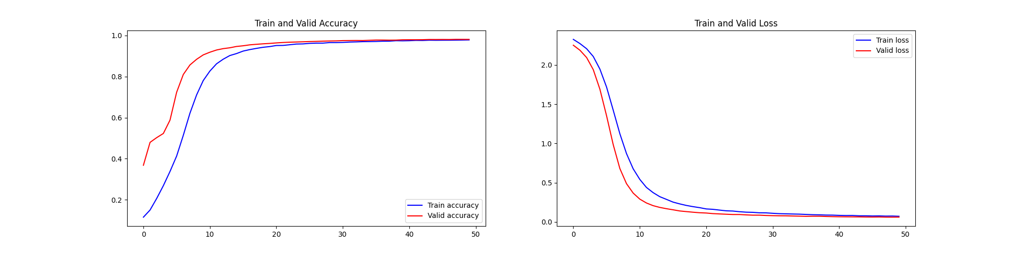
前十个图片对应的标签：　
 [7 2 1 0 4 1 4 9 5 9]

取前十张图片测试集预测：
 [7 2 1 0 4 1 4 9 5 9]

2、cutoff rate=50% MNIST手写数字识别样本、50epoch - 高质量、中等数量样本

np.shape(X_train_data): (24000, 48, 48, 3)
np.shape(X_test_data): (5000, 48, 48, 3)
np.shape(X_train_val): (6000, 48, 48, 3)
np.shape(Y_train_data): (24000, 10)
np.shape(Y_train_val): (6000, 10)

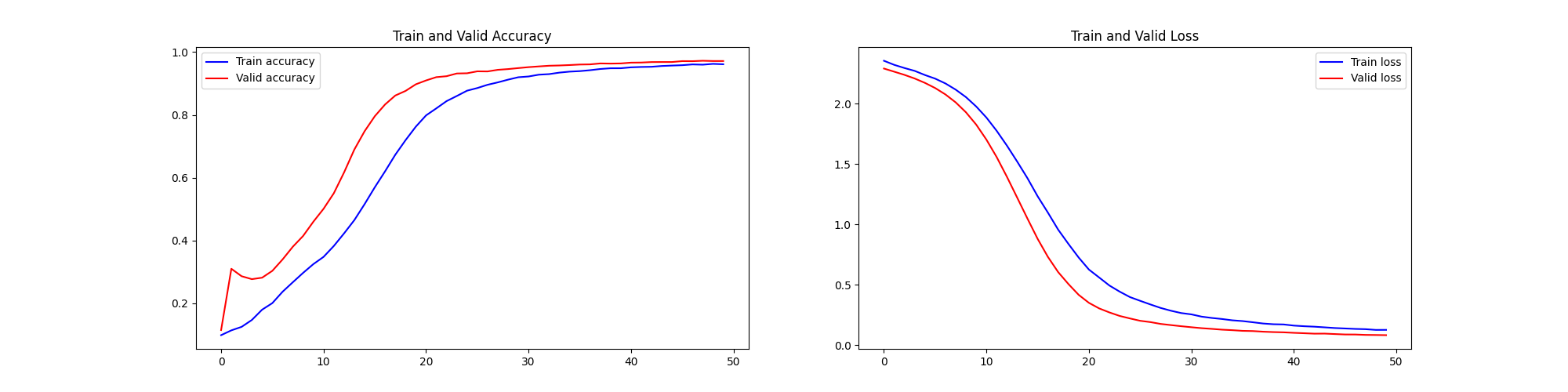
前十个图片对应的标签：　
 [7 2 1 0 4 1 4 9 5 9]

取前十张图片测试集预测：
 [7 2 1 0 4 1 4 9 5 9]

3、cutoff rate=10% MNIST手写数字识别样本、50epoch - 高质量、较少样本

np.shape(X_train_data): (4800, 48, 48, 3)
np.shape(X_test_data): (1000, 48, 48, 3)
np.shape(X_train_val): (1200, 48, 48, 3)
np.shape(Y_train_data): (4800, 10)
np.shape(Y_train_val): (1200, 10)

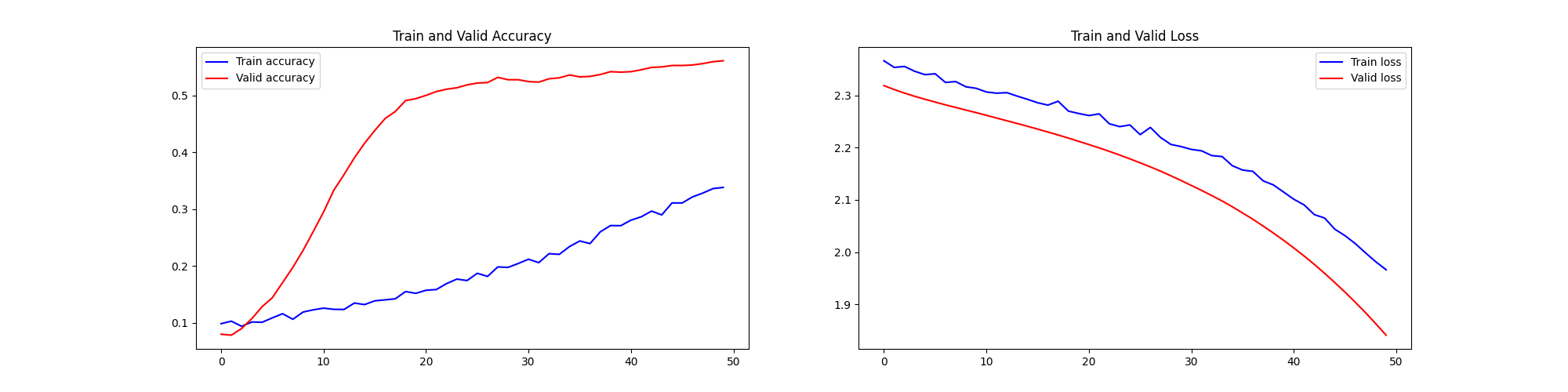
前十个图片对应的标签：　
 [7 2 1 0 4 1 4 9 5 9]

取前十张图片测试集预测：
 [7 2 1 0 4 1 4 9 5 9]

4、cutoff rate=2.5% MNIST手写数字识别样本、50epoch - 高质量、少量样本

np.shape(X_train_data): (1200, 48, 48, 3)
np.shape(X_test_data): (250, 48, 48, 3)
np.shape(X_train_val): (300, 48, 48, 3)
np.shape(Y_train_data): (1200, 10)
np.shape(Y_train_val): (300, 10)

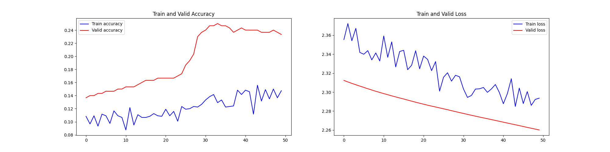
前十个图片对应的标签：　
 [7 2 1 0 4 1 4 9 5 9]
 
取前十张图片测试集预测：
 [7 2 1 0 4 1 4 9 5 9]

5、cutoff rate=2.5% MNIST手写数字识别样本、1000epoch - 高质量、少量样本、超多轮次训练

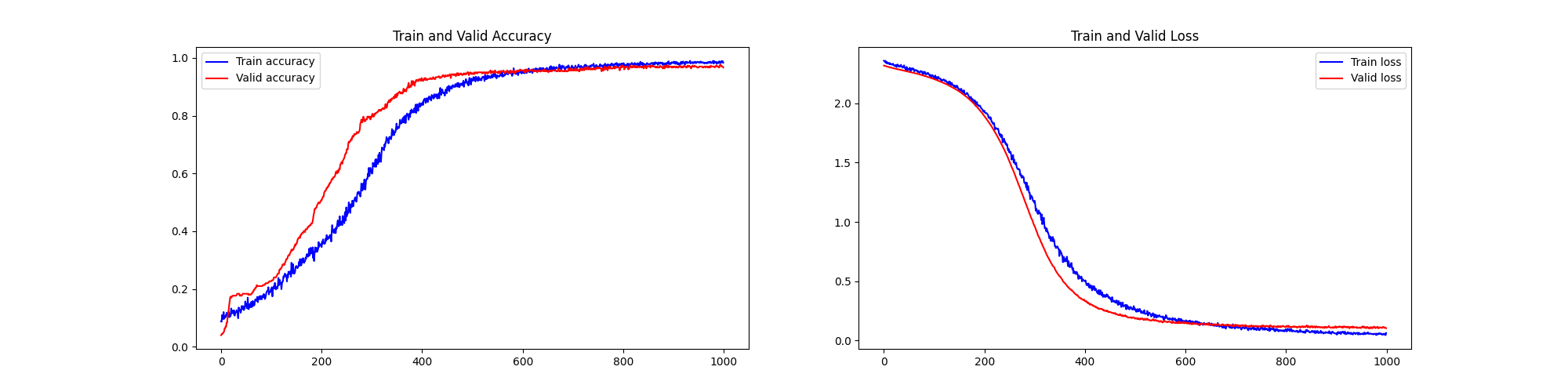
 [7 2 1 0 4 1 4 9 5 9]
 
取前十张图片测试集预测：
 [7 2 1 0 4 1 4 9 5 9]

6、cutoff rate=1% MNIST手写数字识别样本、2000epoch - 高质量、极少量样本、超多轮次训练

np.shape(X_train_data): (480, 48, 48, 3)
np.shape(X_test_data): (100, 48, 48, 3)
np.shape(X_train_val): (120, 48, 48, 3)
np.shape(Y_train_data): (480, 10)
np.shape(Y_train_val): (120, 10)

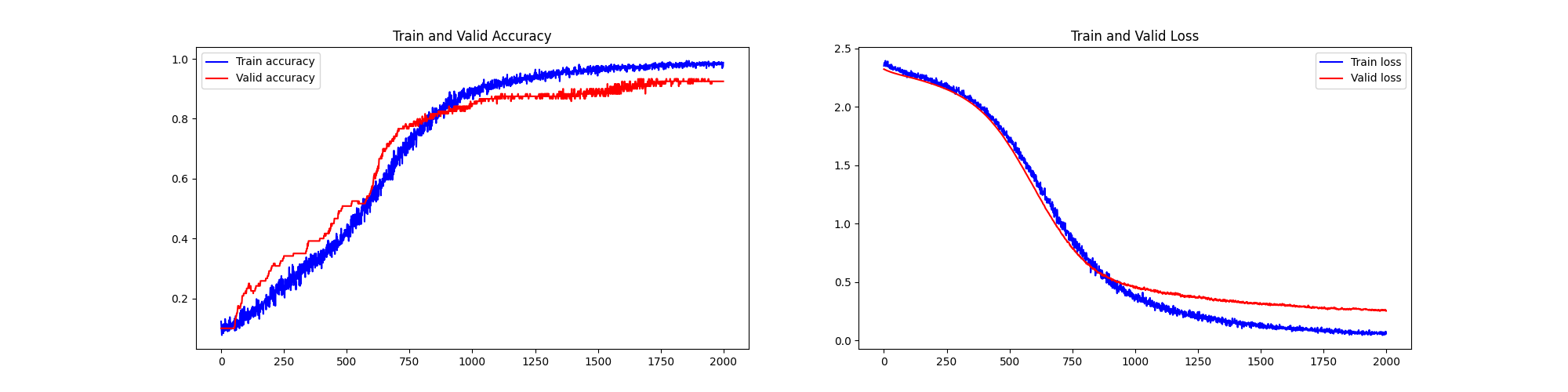
前十个图片对应的标签：　
 [7 2 1 0 4 1 4 9 5 9]
 
取前十张图片测试集预测：
 [7 2 1 0 4 1 4 9 5 9]

7、cutoff rate=0.5% MNIST手写数字识别样本、2000epoch - 高质量、极少量样本、超多轮次训练

np.shape(X_train_data): (240, 48, 48, 3)
np.shape(X_test_data): (50, 48, 48, 3)
np.shape(X_train_val): (60, 48, 48, 3)
np.shape(Y_train_data): (240, 10)
np.shape(Y_train_val): (60, 10)

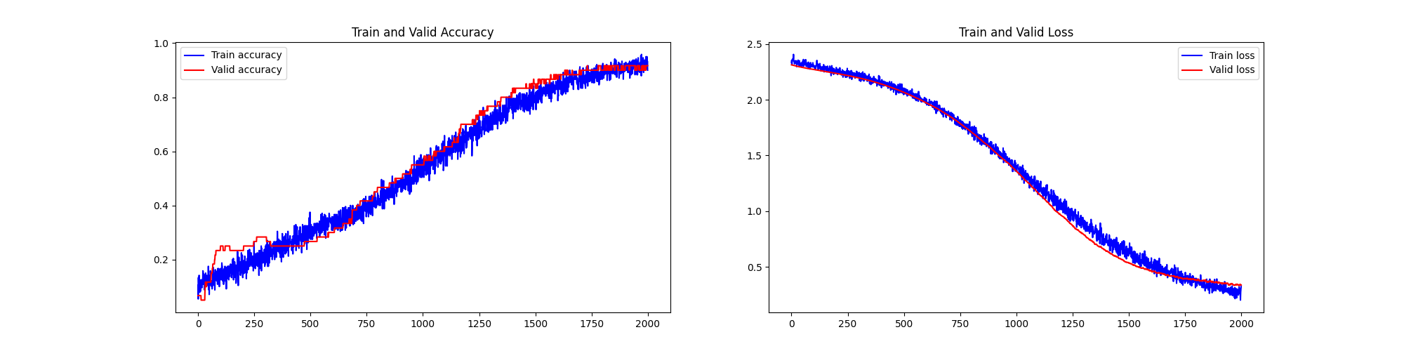
前十个图片对应的标签：　
 [7 2 1 0 4 1 4 9 5 9]
 
取前十张图片测试集预测：
 [7 2 1 0 4 1 4 9 5 9]

8、cutoff rate=0.25% MNIST手写数字识别样本、5000epoch - 高质量、极少量样本、超多轮次训练、更小batchsize、更慢学习速率

np.shape(X_train_data): (120, 48, 48, 3)
np.shape(X_test_data): (25, 48, 48, 3)
np.shape(X_train_val): (30, 48, 48, 3)
np.shape(Y_train_data): (120, 10)
np.shape(Y_train_val): (30, 10)

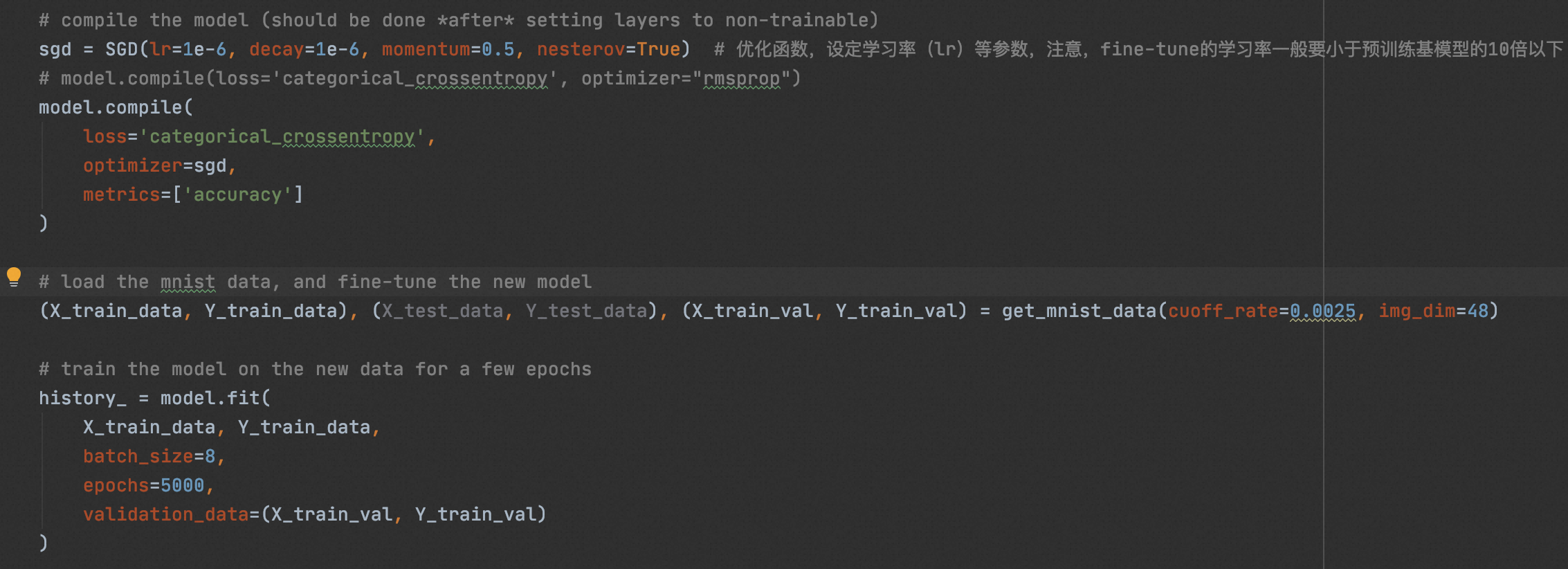
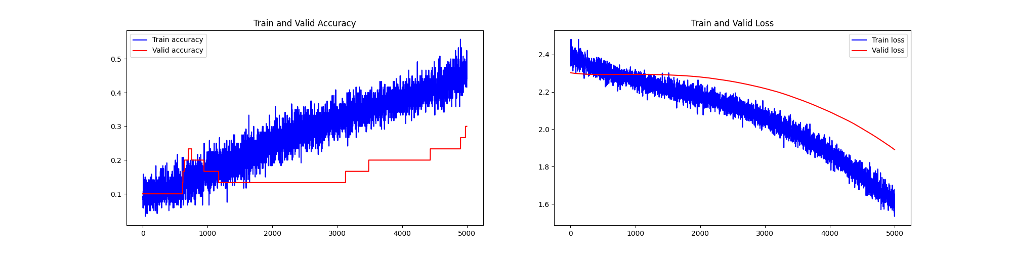
前十个图片对应的标签：　
 [7 2 1 0 4 1 4 9 5 9]

取前十张图片测试集预测：
 [1 1 1 0 1 1 1 1 6 9]

可以看到，当样本量少到一定程度的时候（猜测存在一个样本量临界点），模型的收敛和泛化效果突然产生衰减。

我们尝试两个方向：

轻微加大样本量试试看能不能摸到这个临界点
继续降低学习率和batchsize，尝试获得更好地收敛效果

9、cutoff rate=0.35% MNIST手写数字识别样本、5000epoch - 高质量、极少量样本（轻微加大样本量）、超多轮次训练

np.shape(X_train_data): (168, 48, 48, 3)
np.shape(X_test_data): (35, 48, 48, 3)
np.shape(X_train_val): (42, 48, 48, 3)
np.shape(Y_train_data): (168, 10)
np.shape(Y_train_val): (42, 10)

前十个图片对应的标签：　
 [7 2 1 0 4 1 4 9 5 9]

取前十张图片测试集预测：
 [7 2 1 0 4 1 4 9 2 9]

提高训练样本数量这个方向取得了预期的效果（可能最小样本临界点就在120-150之间），模型的训练收敛和泛化性能都有明显提高。

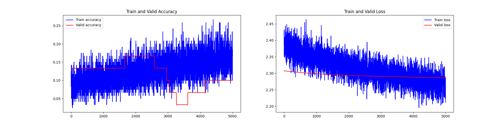
10、cutoff rate=0.25% MNIST手写数字识别样本、5000epoch - 高质量、极少量样本（样本量不变）、超多轮次训练、（继续降低学习率和batchsize）

np.shape(X_train_data): (120, 48, 48, 3)
np.shape(X_test_data): (25, 48, 48, 3)
np.shape(X_train_val): (30, 48, 48, 3)
np.shape(Y_train_data): (120, 10)
np.shape(Y_train_val): (30, 10)

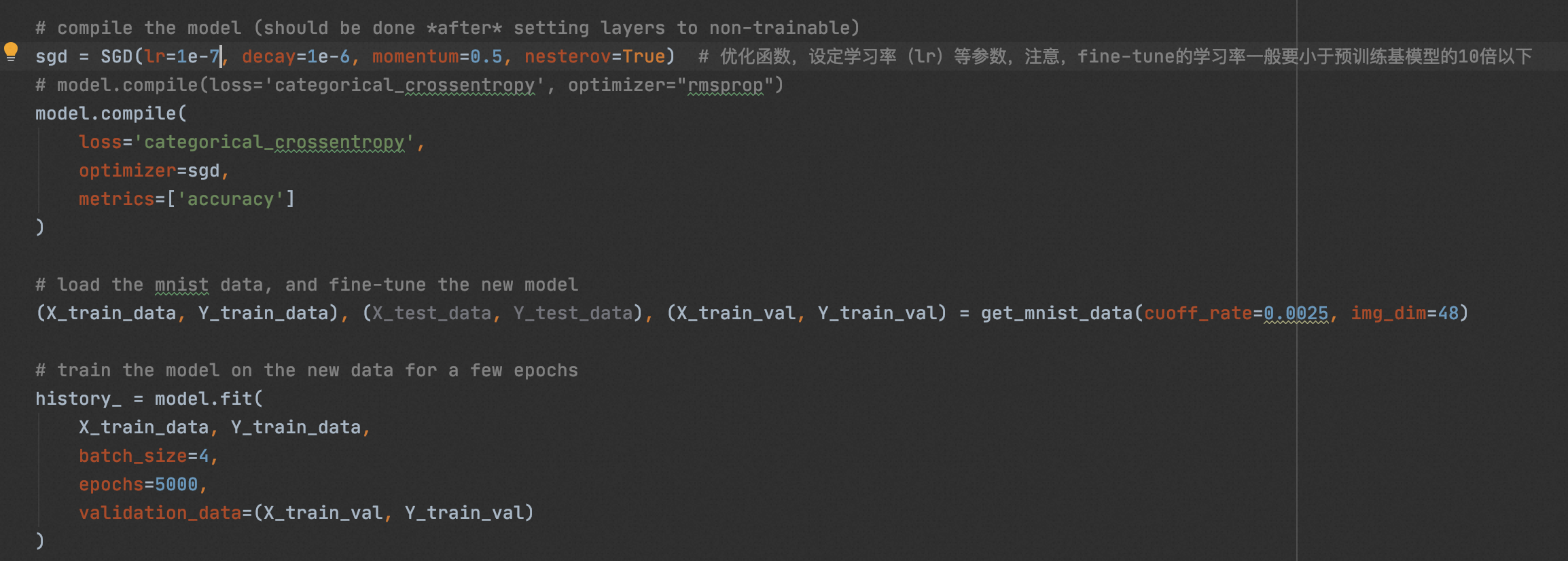
前十个图片对应的标签：　
 [7 2 1 0 4 1 4 9 5 9]

取前十张图片测试集预测：
 [0 0 1 0 0 1 0 0 0 0]

可以看到，在样本量未到达”最小样本临界点“的时候，不管采用多低的学习率和更新率，模型的收敛性能和泛化性能都很差。

结论总结：

预训练后的基模型是一个非常关键的因素，预训练基模型起到了一个”指导方向“的作用。如果没有基模型先前的充分预训练，在fine-tune的时候很容易受到样本数量不足、训练轮次不足等因素的影响，从而导致过拟合或者欠拟合问题的发生。换句话说，基模型本身需要喂入海量高质量的样本，以完成必要的优化方向探索和收敛稳定过程。
在fine-tune任务中，有几个因素起到主要更关键作用
- 多样性：更好地多样性可以显著提升模型的性能
- 质量：即样本纯净度，对模型的收敛和性能存在显著性影响
- BP update size：在样本量较少的时，降低batchsize有助于提升收敛性能
- 梯度学习率：在样本量较少的时，降低learning rate有助于提升收敛性能
在收敛速度合适、批次大小合理、训练轮次足够多、样本多样性和质量足够好的前提下，样本数量对模型收敛和泛化性不存在明显地制约效果。但是样本数量也不能无限降低，存在一个”最小样本临界点“，猜测可能和概率分布典型集原理有关（只要覆盖超过3标准差概率分布的少量典型集就可以提供足够的概率分布信息？笔者曾经有过类似的猜想。）。当超过最小样本临界点后，继续增加样本的收益是边际递减的。在样本量未到达”最小样本临界点“的时候，不管采用多低的学习率和更新率，模型的收敛性能和泛化性能都很差。
一个可能的方向性暗示：对齐的规模法则不必然只受数量影响，而更可能是在保持高质量响应的同时，提升提示的多样性，同时保证超过最小样本临界点即可。

参考链接：

https://arxiv.org/pdf/1409.1556.pdf 
https://www.cnblogs.com/LittleHann/p/6792511.html 
https://github.com/xiaochus/VisualizationCNN/blob/master/vis.py 
https://www.quora.com/What-is-the-VGG-neural-network 
https://blog.csdn.net/wphkadn/article/details/86772708
https://zhuanlan.zhihu.com/p/483559442 
https://keras.io/api/applications/
https://blog.csdn.net/newlw/article/details/126127251 
https://www.image-net.org/challenges/LSVRC/index.php
https://www.cnblogs.com/chentiao/p/16351380.html

三、通过VGG16迁移学习探寻基模型fine-tune/训练级驱动对齐技术的基本原理和应用边界条件

本章节，我们要通过实验探寻几个问题：

本质上，fine-tune所使用的语料是基模型所使用的语料的一个子集，可以理解为条件概率预测空间更小了。如果允许基模型参数调整，是否因为fine-tune的语料概率预测空间变小了，会导致fine-tune后基模型出现“能力退化，并向新领域任务重发展”？或者说，基模型完成迁移学习的代价是否就是“能力退化，并向新领域任务重发展”？
在不改变输入层和输出层的张量维度的前提下，基模型+下游模型stacking后的新模型，分别考察“允许基模型参数调整”和“不允许基模型参数调整”两种情况下，在使用一份新的领域任务语料进行训练后，整体模型的迁移学习效果如何？

整体方案设计原理如下：

本质上，大模型的fine-tune是在做新语料的自监督学习，和传统有监督学习在原理上是类似的，只是因为模型结构的不同，导致监督反馈的方式有所不同。所以该实验一定程度上可以揭示大模型fine-tune-align的基本原理。
当前的大模型应用场景中，最流行的范式就是大模型+fine-tune，从模型层面看，这种范式的本质就是：不改变输入层和输出层的张量维度（模型结构整体结构不变），用一份新的领域任务数据喂入模型（训练集驱动对齐技术），根据基模型对新任务的迁移泛化能力，决定是否以及freeze多少层基模型的参数，然后对stacking后的模型进行再次训练。
“新任务”是绝对意义上的新任务，即新任务领域数据集和基模型训练集的相似度很小。因此本实验中所使用的基模型是VGG16（使用imageNet 1000训练得到），新领域数据是MNIST手写数字。这模拟了在应用大模型时，下游任务往往具备一些垂直属性，和大模型的训练语料库存在较大的不同，但同时它们又都是像素图片，所以又没有完全脱离基模型的先验假设，一定程度上，这可以模拟NLP大模型在进行文本生成领域应用的场景。

0x1：实验一：可视化VGG16各层卷积层

测试图片如下：

6.webp

elephant.png

MNIST数字图片 7_224

VGG16对这3张图的预测结果如下：

6.webp
Predicted: [('n03532672', 'hook', 0.4591384), ('n02910353', 'buckle', 0.032941677), ('n01930112', 'nematode', 0.032439113)]

elephant.png
Predicted: [('n02504458', 'African_elephant', 0.6726845), ('n01871265', 'tusker', 0.17410518), ('n02504013', 'Indian_elephant', 0.054779347)]

7_244.png
Predicted: [('n04118776', 'rule', 0.8002465), ('n06359193', 'web_site', 0.08262307), ('n03782006', 'monitor', 0.015786884)]

可以看到，3张图都预测错了，VGG16的只能按照ImageNet1000的训练集进行泛化预测，对没有见过的样本，只能给出尝试性的近似预测。

可视化在6.webp输入下的卷积层，

conv_block1_conv1

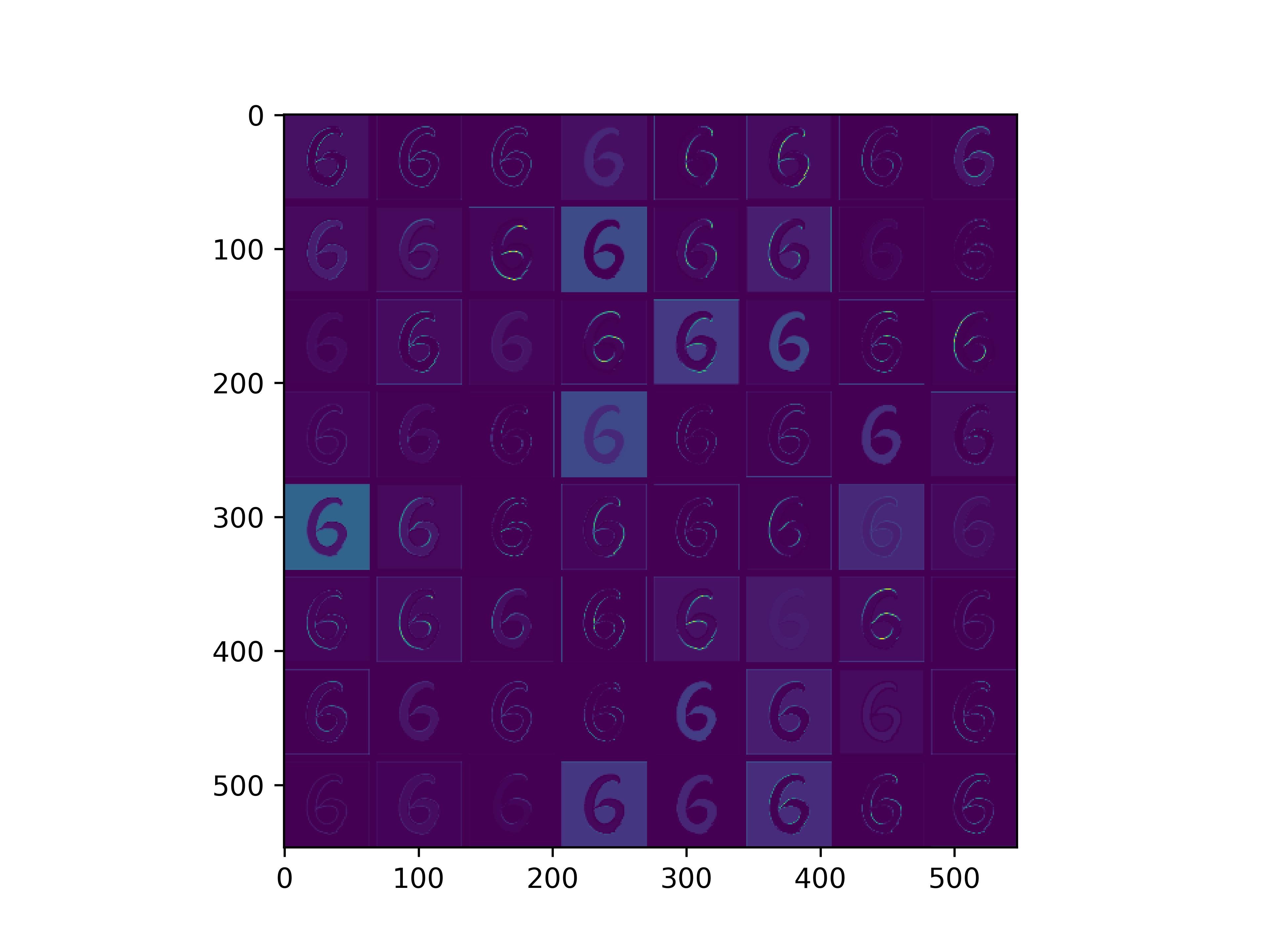
conv_block1_conv2

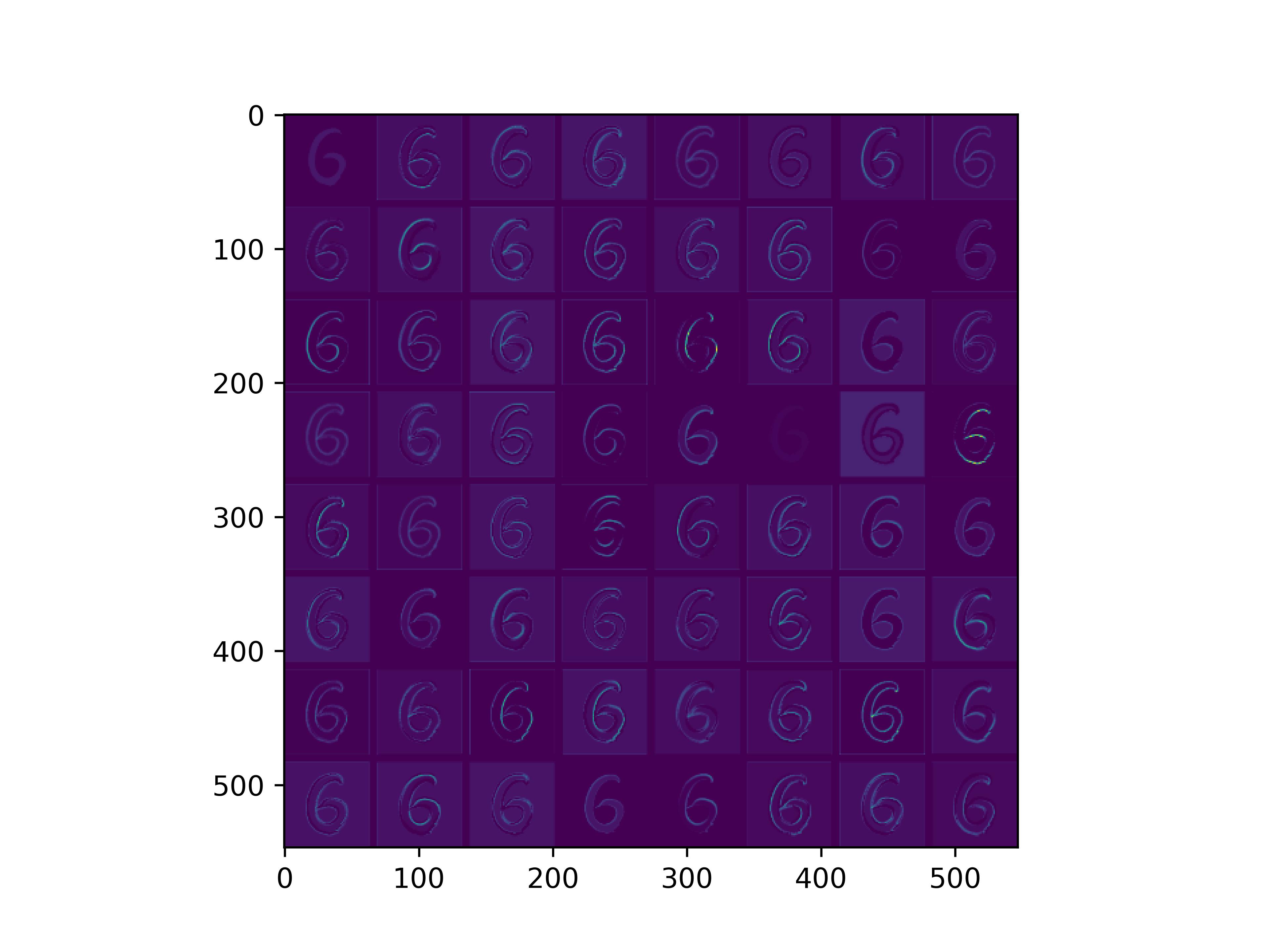
conv_block2_conv1

conv_block2_conv2

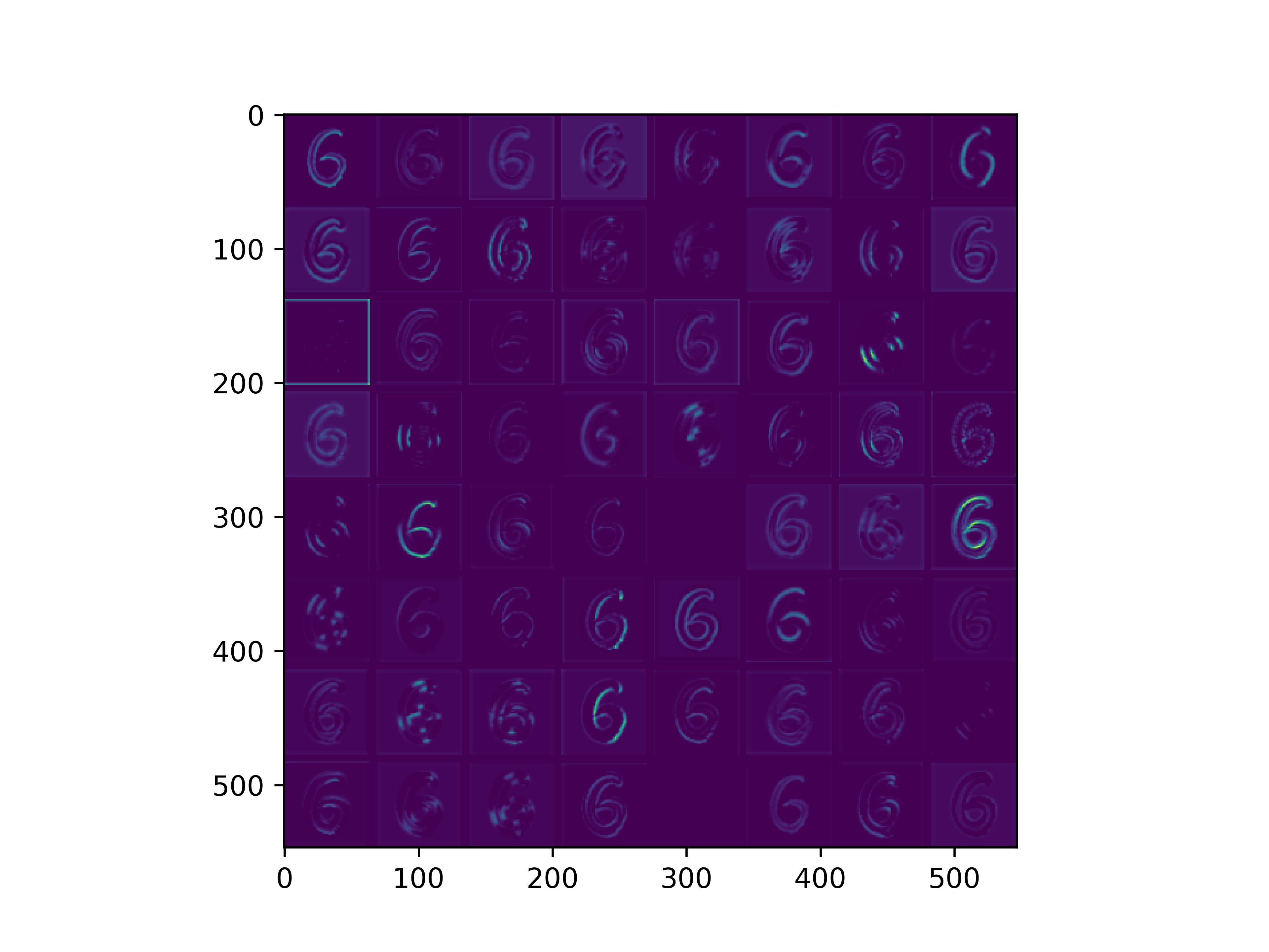
conv_block3_conv1

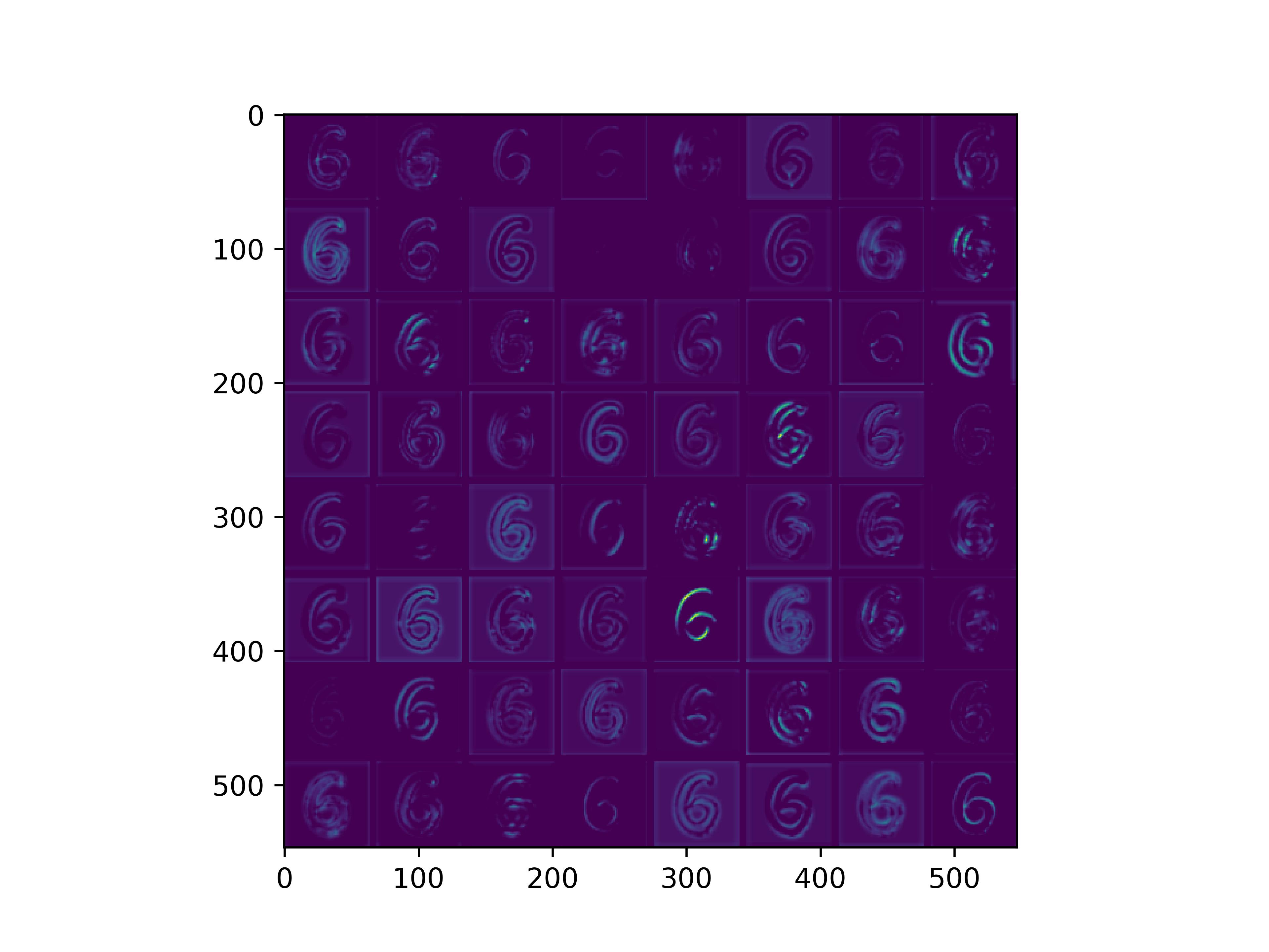
conv_block3_conv2

conv_block5_conv3

可视化在elephant.png输入下的卷积层，

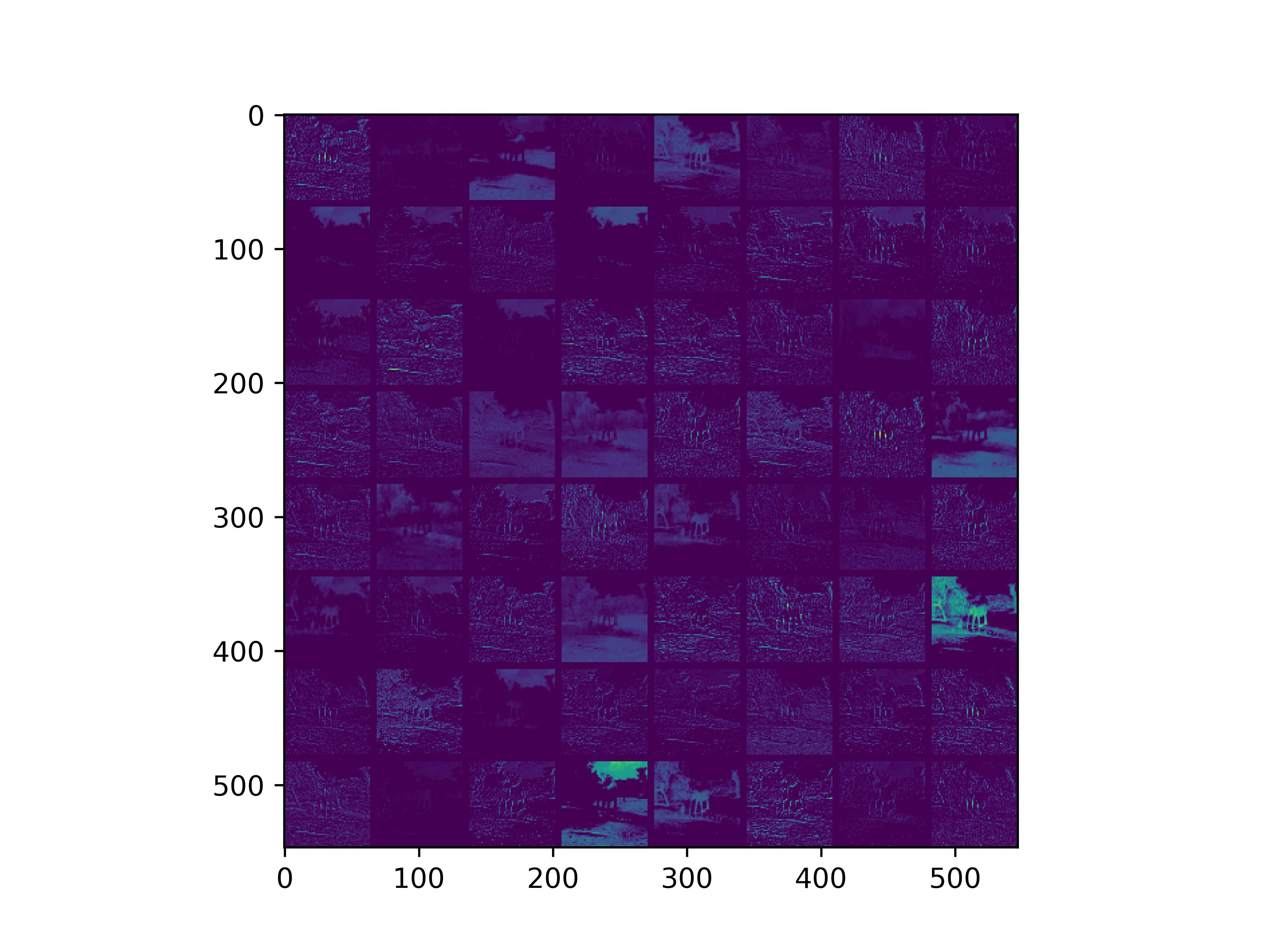
conv_block1_conv1

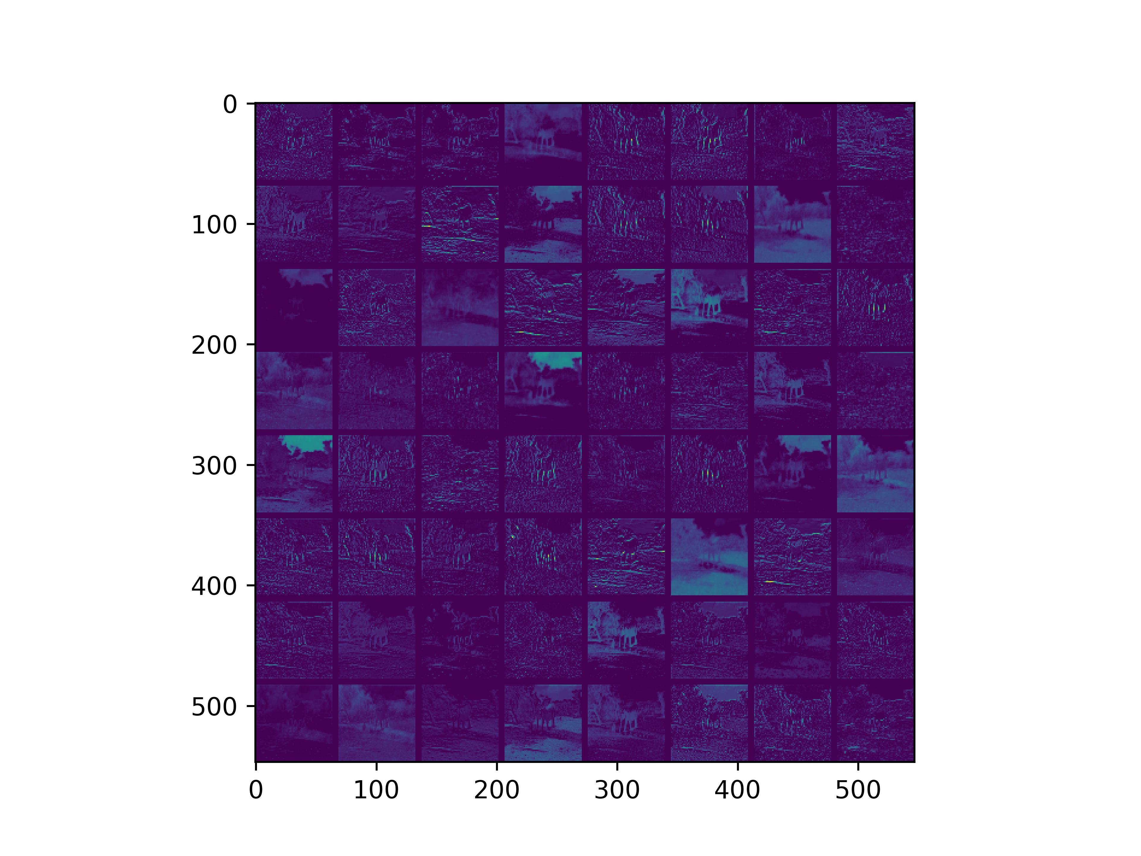
conv_block1_conv2

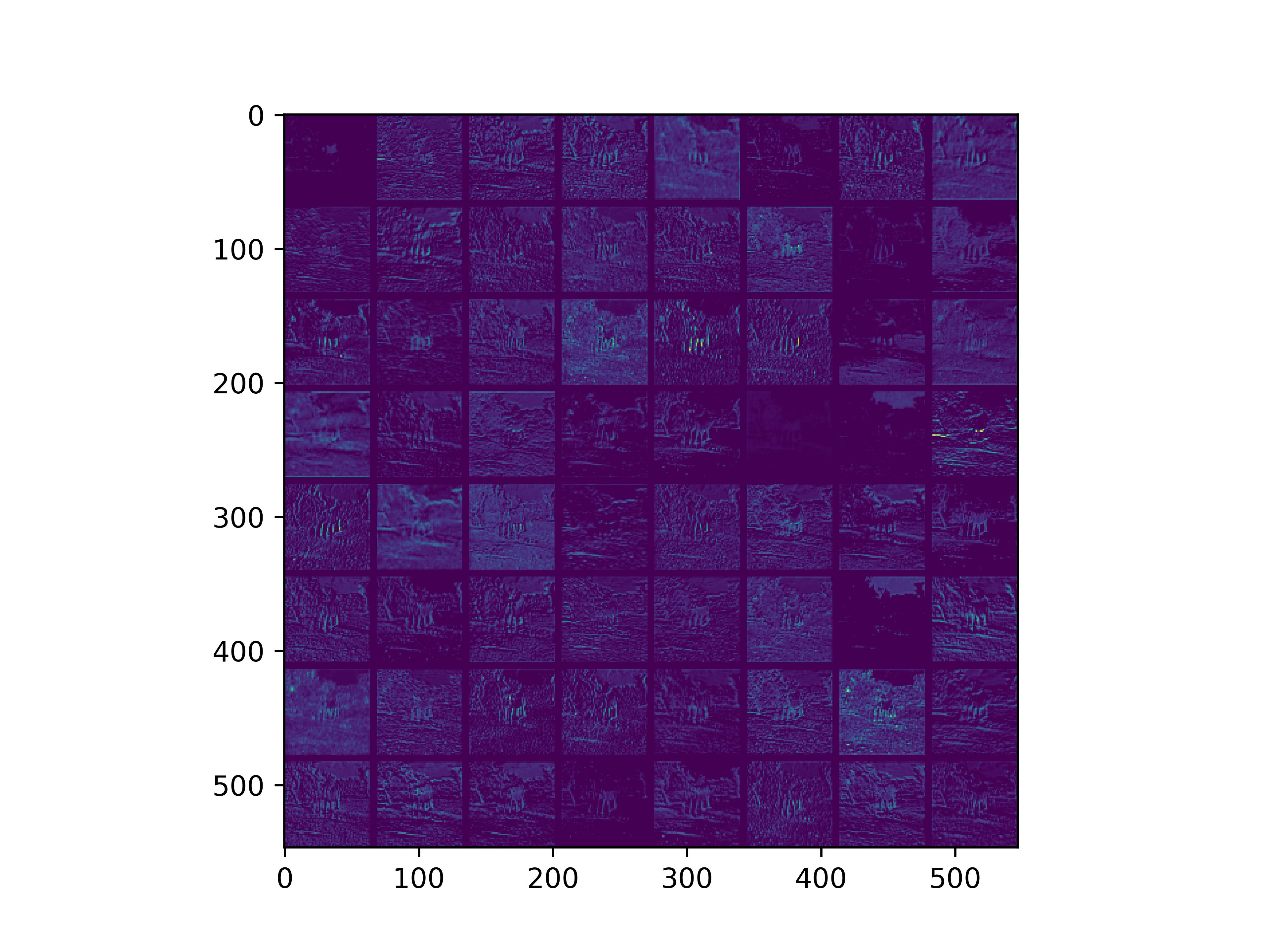
conv_block2_conv1

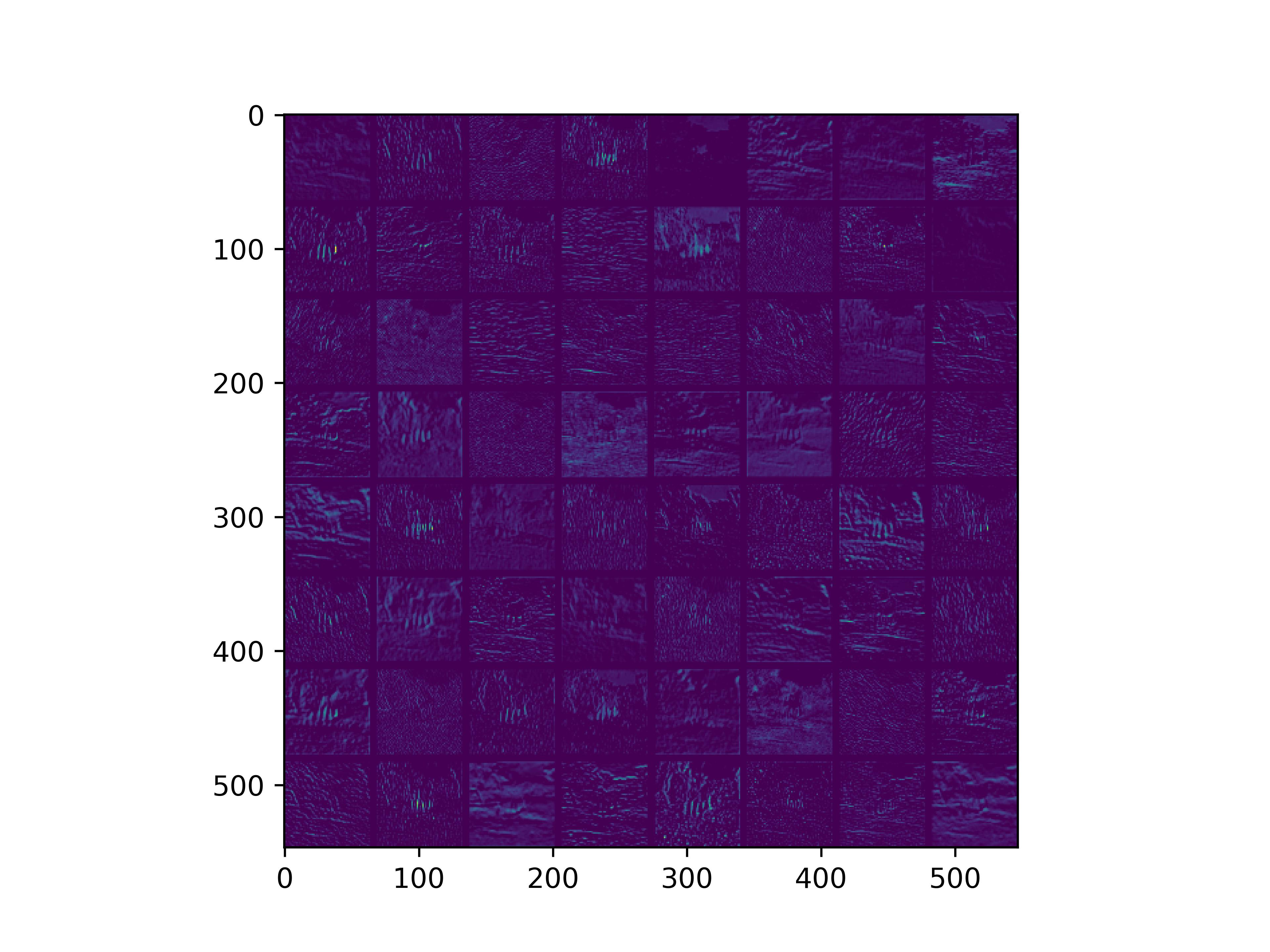
conv_block2_conv2

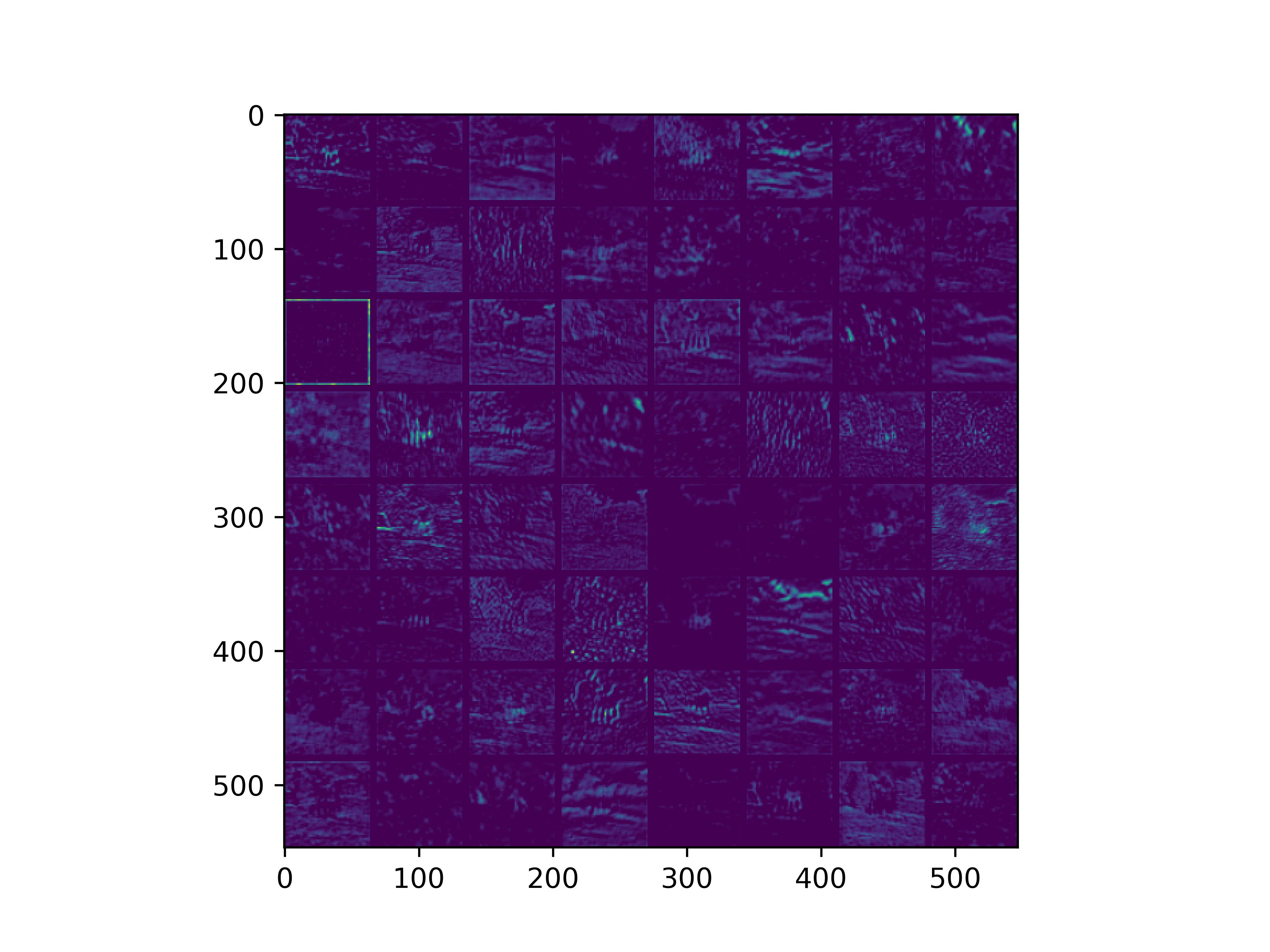
conv_block3_conv1

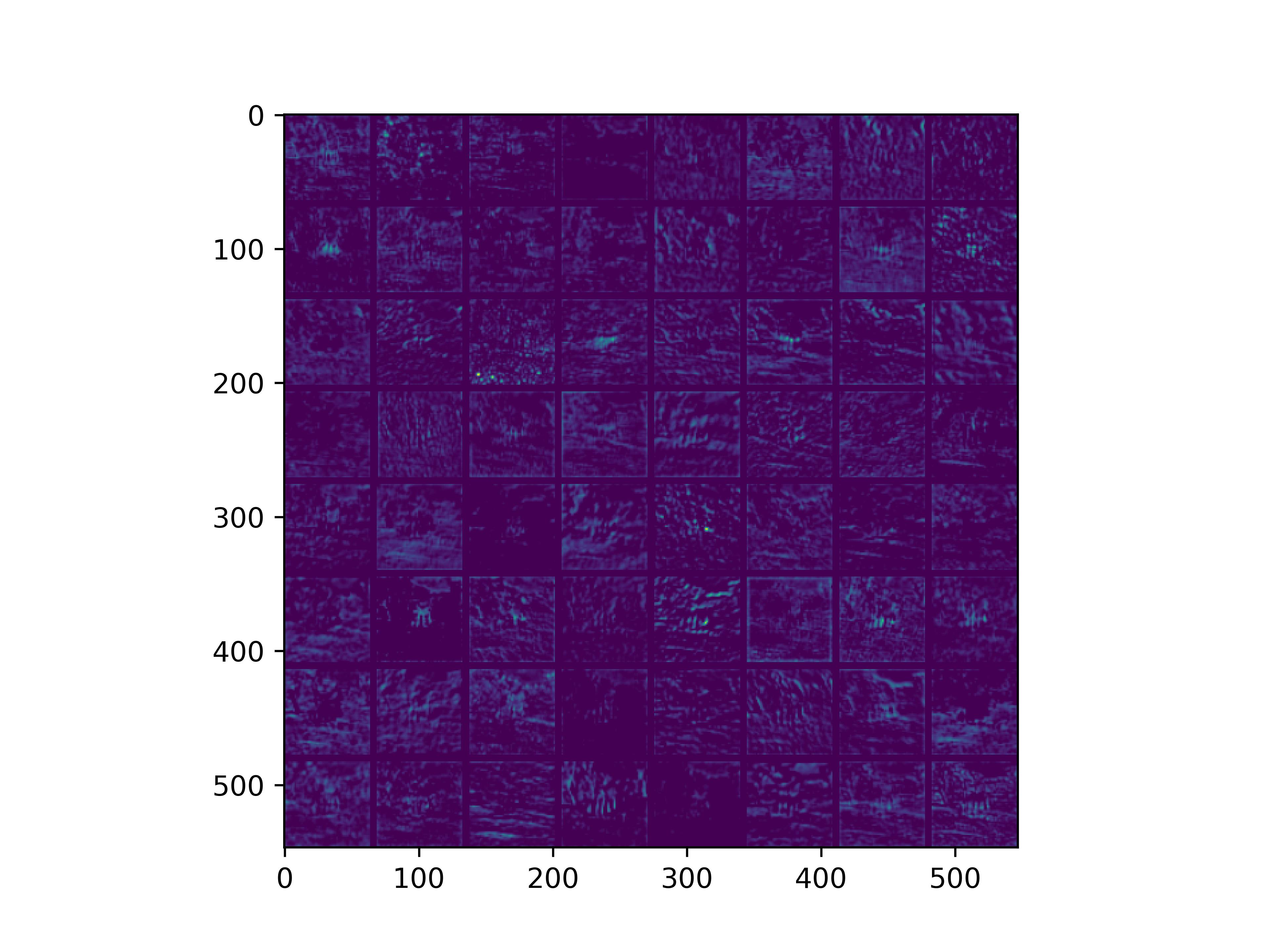
conv_block3_conv2

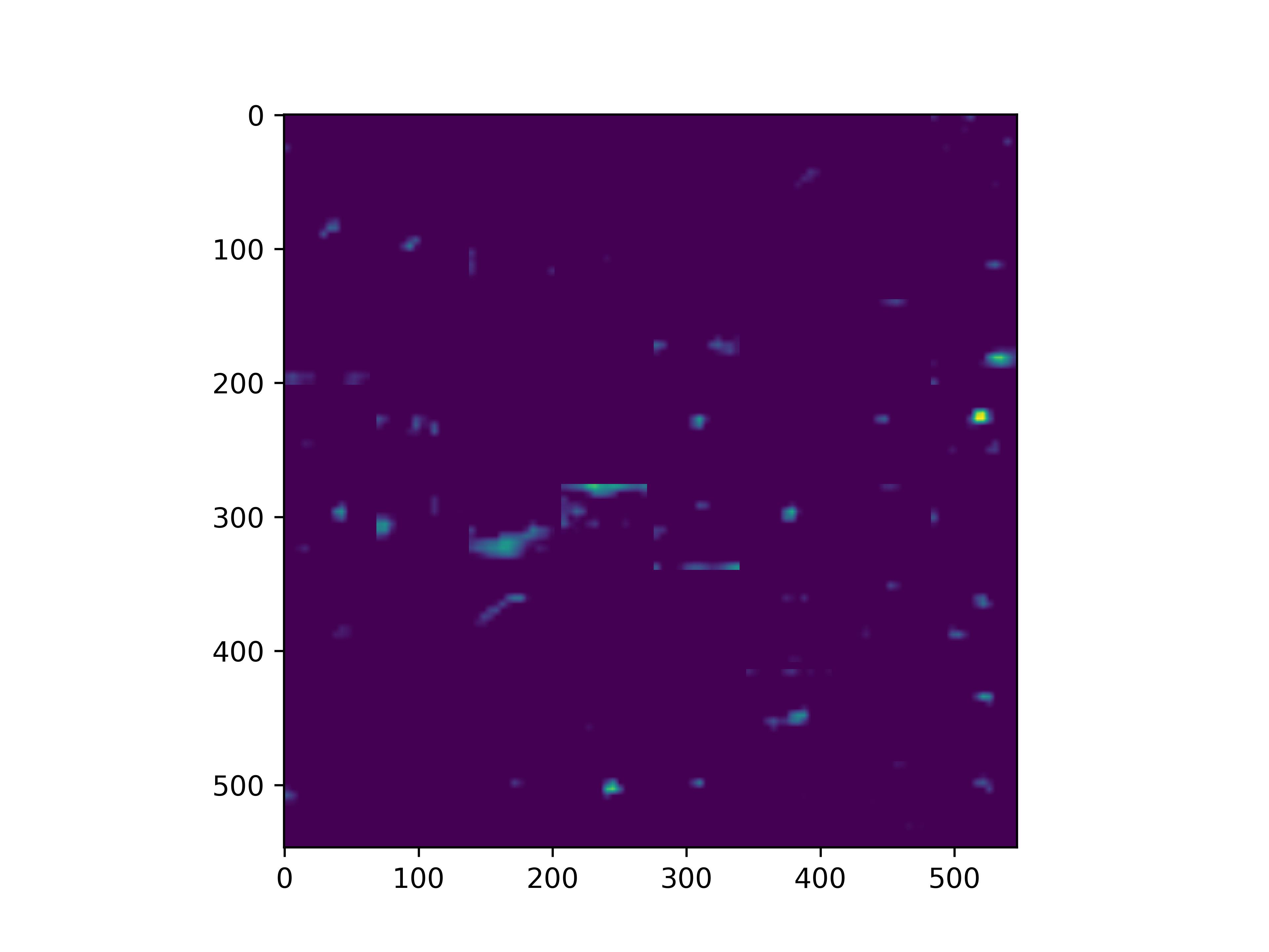
conv_block5_conv3

可视化在7_244.png输入下的卷积层，

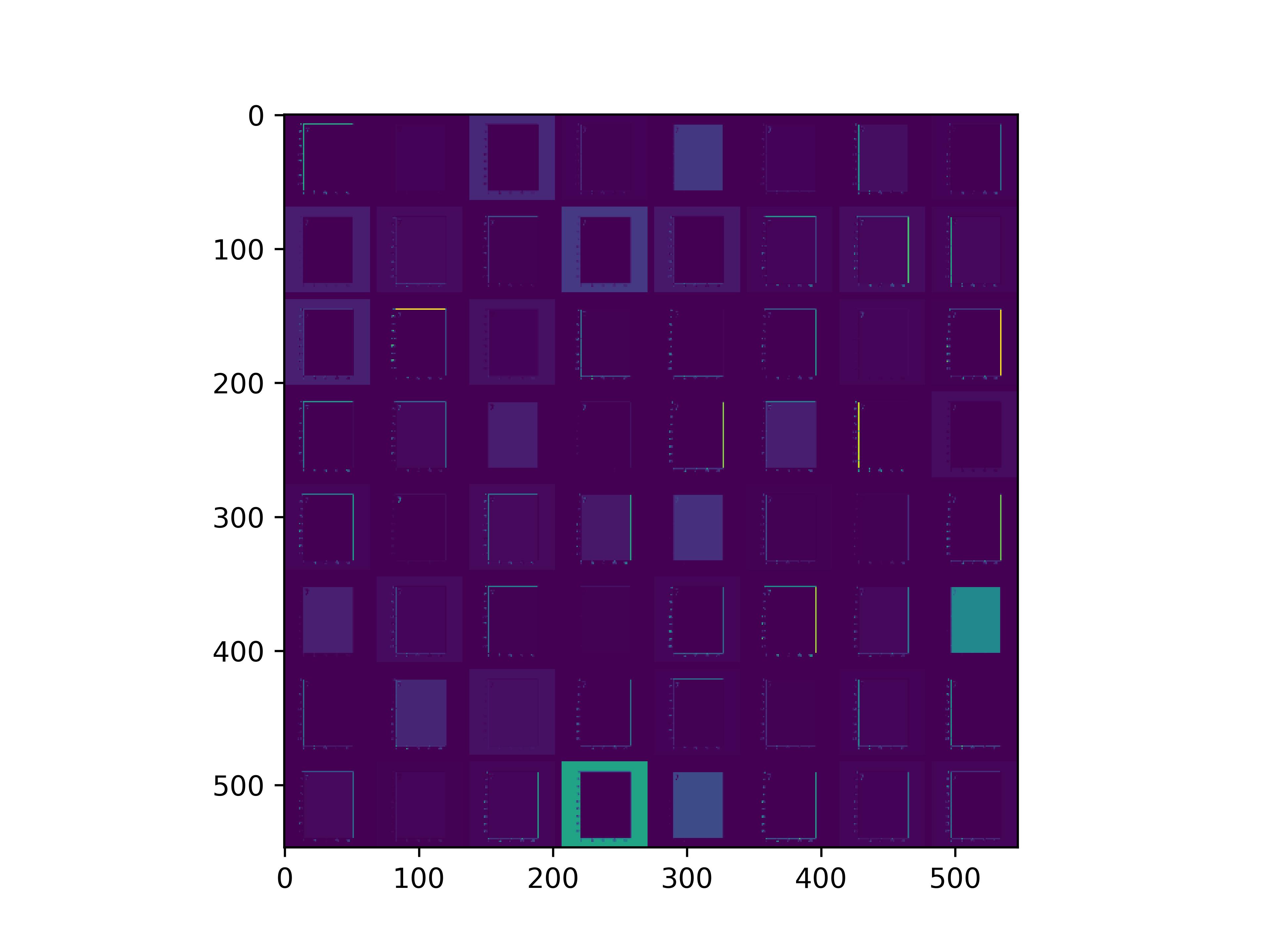
conv_block1_conv1

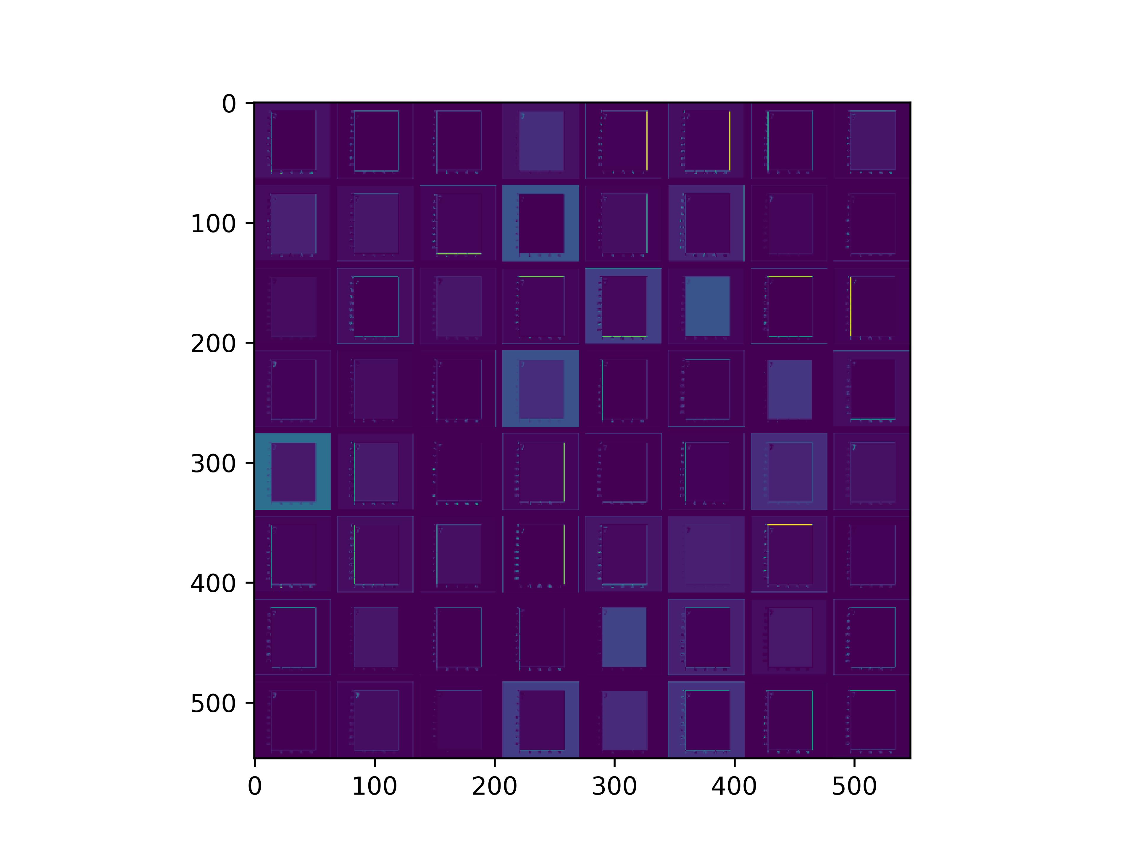
conv_block1_conv2

conv_block2_conv1

conv_block2_conv2

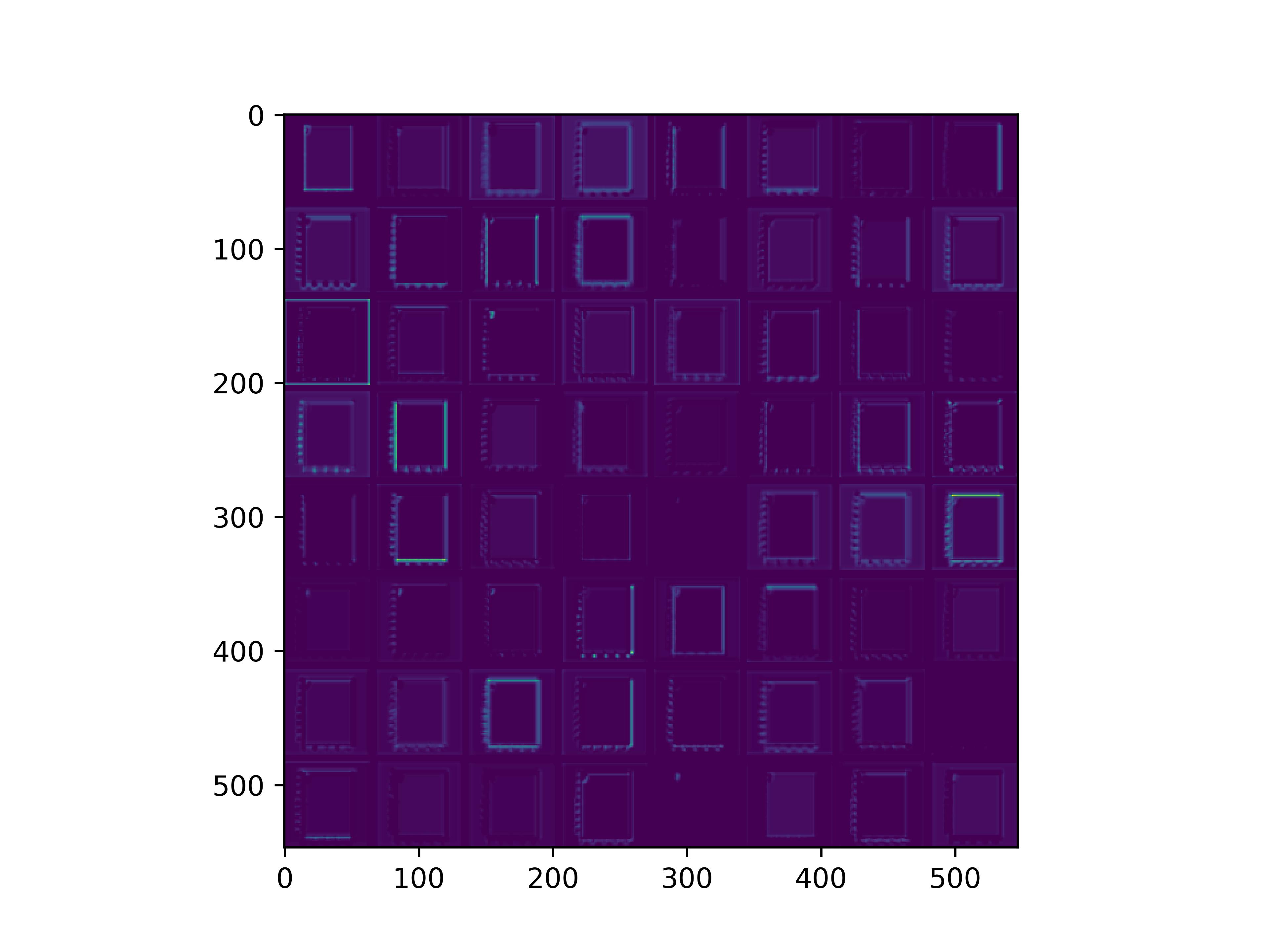
conv_block3_conv1

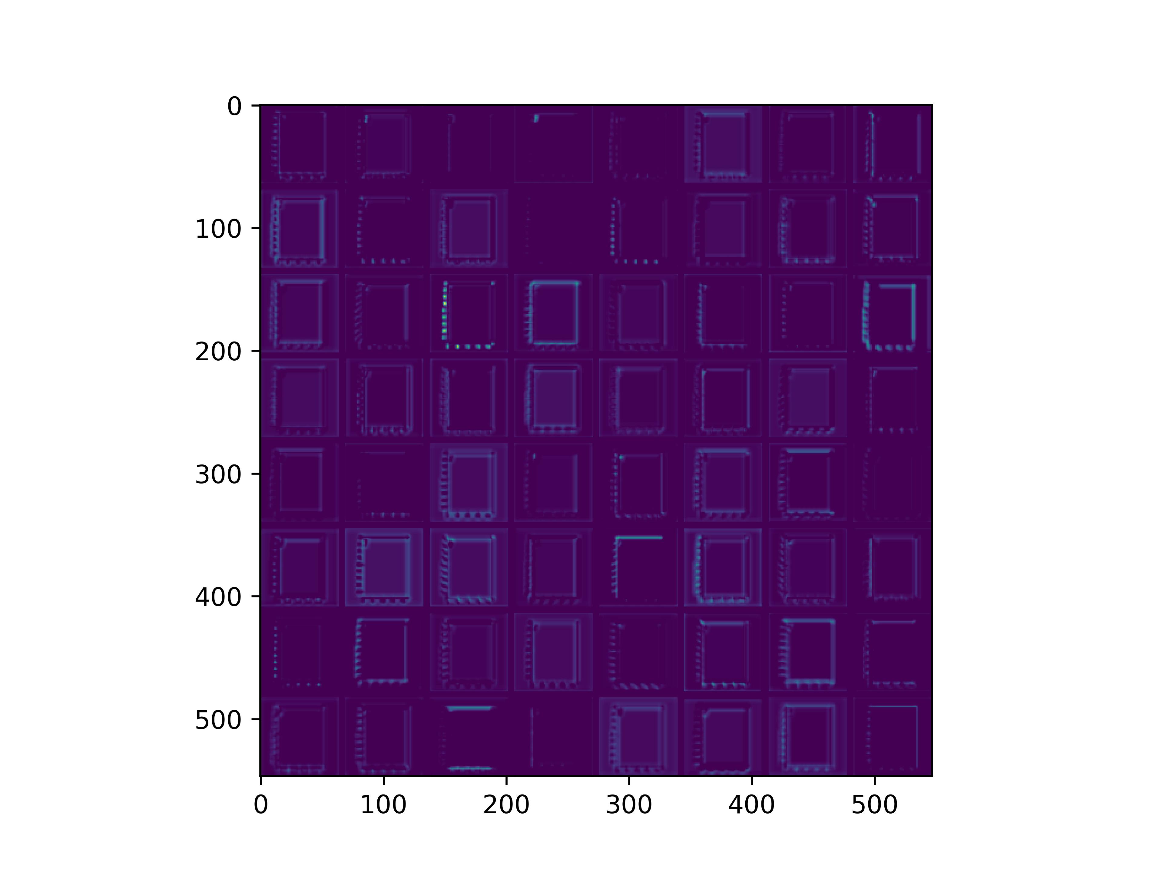
conv_block3_conv2

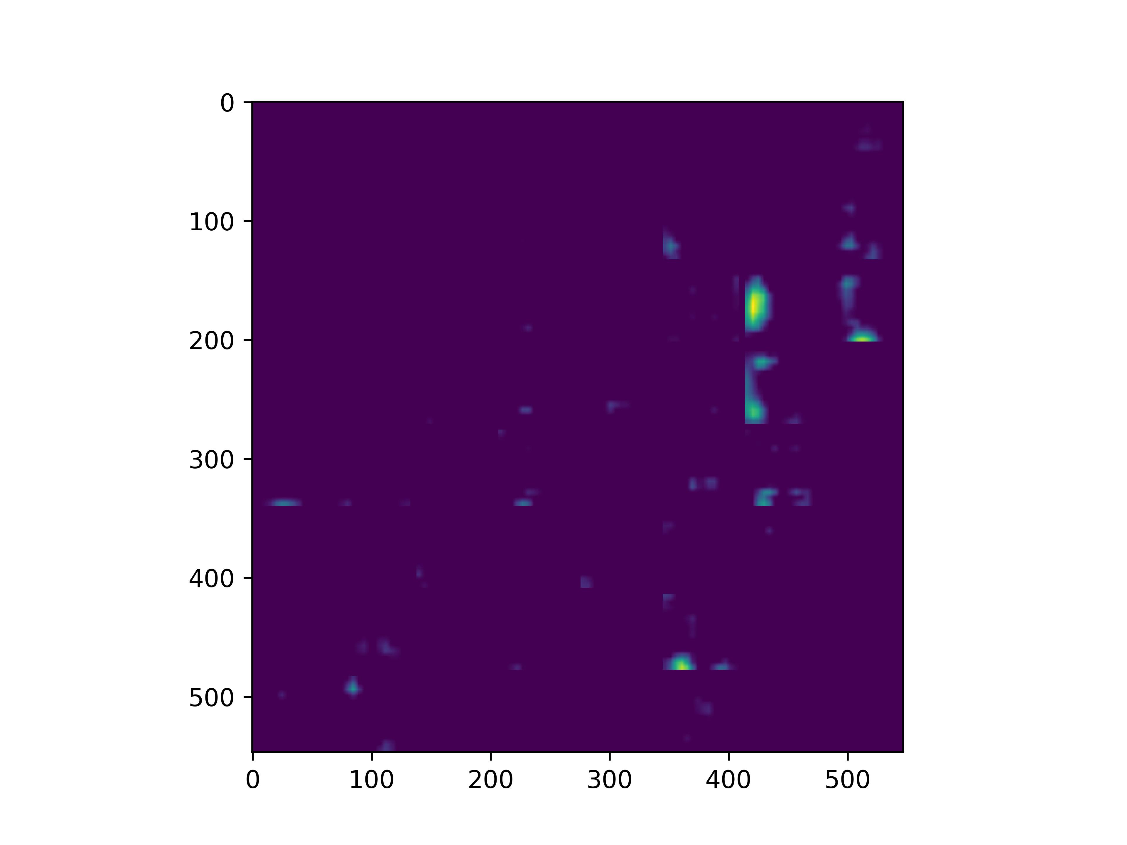
conv_block5_conv3

0x2：实验二：在预训练基模型的基础上，基模型参数freeze，stacking一个新的下游模型，不改变输入层和输出层的张量维度。输入MNIST手写数字图片样本（和VGG16使用的Imagenet1000存在相似但也有不同的地方）进行fine-tune训练，探寻该条件下fine-tune模型对新领域任务的迁移能力以及对原始任务的衰退现象

模型结构如下：

base_model.input_shape:  (None, 224, 224, 3)
base_model.input_shape[1:]:  (224, 224, 3)
base_model.output_shape:  (None, 7, 7, 512)
base_model.output_shape[1:]:  (7, 7, 512)
model.input_shape:  (None, 224, 224, 3)
model.input_shape[1:]:  (224, 224, 3)
model.output_shape:  (None, 1000)
model.output_shape[1:]:  (1000,)
Model: "model"
_________________________________________________________________
 Layer (type)                Output Shape              Param #   
=================================================================
 input_1 (InputLayer)        [(None, 224, 224, 3)]     0         
                                                                 
 block1_conv1 (Conv2D)       (None, 224, 224, 64)      1792      
                                                                 
 block1_conv2 (Conv2D)       (None, 224, 224, 64)      36928     
                                                                 
 block1_pool (MaxPooling2D)  (None, 112, 112, 64)      0         
                                                                 
 block2_conv1 (Conv2D)       (None, 112, 112, 128)     73856     
                                                                 
 block2_conv2 (Conv2D)       (None, 112, 112, 128)     147584    
                                                                 
 block2_pool (MaxPooling2D)  (None, 56, 56, 128)       0         
                                                                 
 block3_conv1 (Conv2D)       (None, 56, 56, 256)       295168    
                                                                 
 block3_conv2 (Conv2D)       (None, 56, 56, 256)       590080    
                                                                 
 block3_conv3 (Conv2D)       (None, 56, 56, 256)       590080    
                                                                 
 block3_pool (MaxPooling2D)  (None, 28, 28, 256)       0         
                                                                 
 block4_conv1 (Conv2D)       (None, 28, 28, 512)       1180160   
                                                                 
 block4_conv2 (Conv2D)       (None, 28, 28, 512)       2359808   
                                                                 
 block4_conv3 (Conv2D)       (None, 28, 28, 512)       2359808   
                                                                 
 block4_pool (MaxPooling2D)  (None, 14, 14, 512)       0         
                                                                 
 block5_conv1 (Conv2D)       (None, 14, 14, 512)       2359808   
                                                                 
 block5_conv2 (Conv2D)       (None, 14, 14, 512)       2359808   
                                                                 
 block5_conv3 (Conv2D)       (None, 14, 14, 512)       2359808   
                                                                 
 block5_pool (MaxPooling2D)  (None, 7, 7, 512)         0         
                                                                 
 flatten (Flatten)           (None, 25088)             0         
                                                                 
 dense (Dense)               (None, 4096)              102764544 
                                                                 
 dropout (Dropout)           (None, 4096)              0         
                                                                 
 dense_1 (Dense)             (None, 4096)              16781312  
                                                                 
 dropout_1 (Dropout)         (None, 4096)              0         
                                                                 
 dense_2 (Dense)             (None, 1000)              4097000   
                                                                 
=================================================================
Total params: 138,357,544
Trainable params: 138,357,544
Non-trainable params: 0

原始MNIST的X训练集和Y标签集都需要进行适配改造，

input：28,28 -> 224,224,3
output：10 -> 1000

    (X_train_data, Y_train_data), (X_test_data, Y_test_data) = mnist.load_data()
    # Y_train_data = reshape(Y_train_data[:5], (None,1000))
    print("np.shape(Y_train_data): ", np.shape(Y_train_data))
    print("Y_train_data: ", Y_train_data)
    Y_train_data = to_categorical(Y_train_data)
    print("Y_train_data: ", Y_train_data)

    Y_train_data = concatenate((Y_train_data, np.zeros((np.shape(Y_train_data)[0], 990))), axis=1)
    print("Y_train_data: ", Y_train_data)
    print("np.shape(Y_train_data): ", np.shape(Y_train_data))

对原有MNIST的10维标签集进行扩展到1000维，从10维以后的bit位填0。

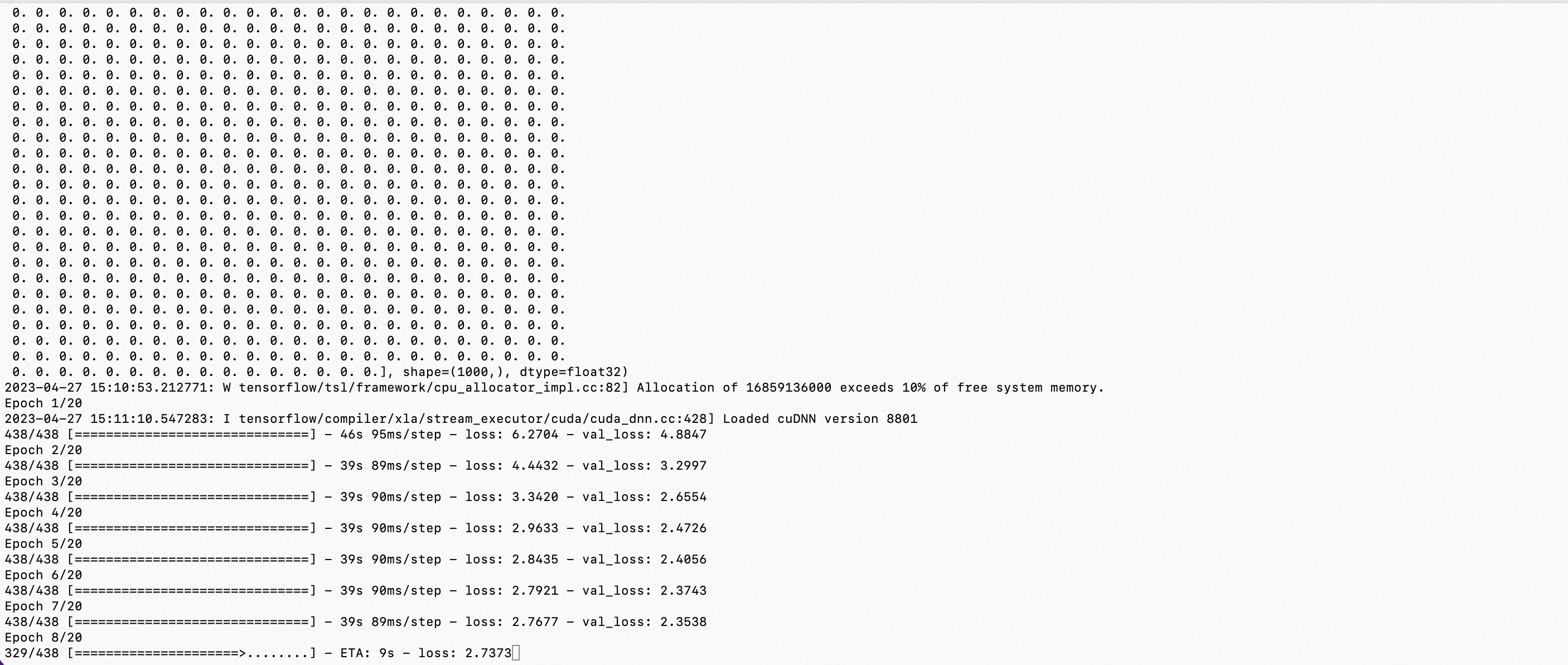
训练过程可以看到：

val_loss和loss始终无法收敛
增减样本数量也无法改善收敛情况

使用fine-tune好的模型，对7_224.png（MNIST测试集）进行识别预测，观察迁移学习能力。

from keras.models import Model, load_model
from tensorflow.keras.applications.vgg16 import VGG16
from tensorflow.keras.preprocessing import image
from tensorflow.keras.backend import reshape, expand_dims, spatial_2d_padding, spatial_3d_padding, arange, concatenate
from tensorflow.keras.applications.vgg16 import preprocess_input, decode_predictions
from tensorflow.keras.layers import Dense, GlobalAveragePooling1D, Flatten, Dropout, Conv1D
from keras.optimizers import SGD
from keras.datasets import mnist
from keras.utils import to_categorical
import tensorflow as tf
import numpy as np
import cv2
import matplotlib.pyplot as plt
import pickle

import os
# os.environ["CUDA_VISIBLE_DEVICES"] = "0,1,2,3,4,5,6,7"
os.environ["CUDA_VISIBLE_DEVICES"] = "0"


def vis_conv(images, n, name, t):
    """visualize conv output and conv filter.
    Args:
           img: original image.
           n: number of col and row.
           t: vis type.
           name: save name.
    """
    size = 64
    margin = 5

    if t == 'filter':
        results = np.zeros((n * size + 7 * margin, n * size + 7 * margin, 3))
    if t == 'conv':
        results = np.zeros((n * size + 7 * margin, n * size + 7 * margin))

    for i in range(n):
        for j in range(n):
            if t == 'filter':
                filter_img = images[i + (j * n)]
            if t == 'conv':
                filter_img = images[..., i + (j * n)]
            filter_img = cv2.resize(filter_img, (size, size))

            # Put the result in the square `(i, j)` of the results grid
            horizontal_start = i * size + i * margin
            horizontal_end = horizontal_start + size
            vertical_start = j * size + j * margin
            vertical_end = vertical_start + size
            if t == 'filter':
                results[horizontal_start: horizontal_end, vertical_start: vertical_end, :] = filter_img
            if t == 'conv':
                results[horizontal_start: horizontal_end, vertical_start: vertical_end] = filter_img

    # Display the results grid
    plt.imshow(results)
    plt.savefig('images/{}_{}.jpg'.format(t, name), dpi=600)
    plt.show()


def conv_output(model, layer_name, img):
    """Get the output of conv layer.

    Args:
           model: keras model.
           layer_name: name of layer in the model.
           img: processed input image.

    Returns:
           intermediate_output: feature map.
    """
    # this is the placeholder for the input images
    input_img = model.input

    try:
        # this is the placeholder for the conv output
        out_conv = model.get_layer(layer_name).output
    except:
        raise Exception('Not layer named {}!'.format(layer_name))

    # get the intermediate layer model
    intermediate_layer_model = Model(inputs=input_img, outputs=out_conv)

    # get the output of intermediate layer model
    intermediate_output = intermediate_layer_model.predict(img)

    return intermediate_output[0]


def get_mnist_data(cuoff_rate=1):
    (X_train_data, Y_train_data), (X_test_data, Y_test_data) = mnist.load_data()
    # convert Y label into one-hot
    Y_train_data = to_categorical(Y_train_data)
    Y_test_data = to_categorical(Y_test_data)

    # cutoff by cuoff_rate
    Y_train_data = Y_train_data[:int(np.shape(Y_train_data)[0] * cuoff_rate)]
    Y_test_data = Y_test_data[:int(np.shape(Y_test_data)[0] * cuoff_rate)]
    X_train_data = X_train_data[:int(np.shape(X_train_data)[0] * cuoff_rate), ...]
    X_test_data = X_test_data[:int(np.shape(X_test_data)[0] * cuoff_rate), ...]

    # expand the dim into 1000
    Y_train_data = concatenate((Y_train_data, np.zeros((np.shape(Y_train_data)[0], 990))), axis=1)
    Y_test_data = concatenate((Y_test_data, np.zeros((np.shape(Y_test_data)[0], 990))), axis=1)
    # normalize
    X_train_data = X_train_data.astype('float32') / 255.0
    X_test_data = X_test_data.astype('float32') / 255.0

    # reshape the mnist data in 224*224*3
    X_train_data = expand_dims(X_train_data, axis=-1)
    X_test_data = expand_dims(X_test_data, axis=-1)
    X_train_data = tf.pad(X_train_data, [[0, 0], [2, 194], [2, 194], [1, 1]])
    X_test_data = tf.pad(X_test_data, [[0, 0], [2, 194], [2, 194], [1, 1]])

    # prepare validate/train date
    X_train_val = X_train_data[-2000:, ...]
    X_train_data = X_train_data[:-2000, ...]
    Y_train_val = Y_train_data[-2000:]
    Y_train_data = Y_train_data[:-2000]

    print("np.shape(X_train_data): ", np.shape(X_train_data))
    print("np.shape(X_test_data): ", np.shape(X_test_data))
    print("np.shape(X_train_val): ", np.shape(X_train_val))
    print("np.shape(Y_train_data): ", np.shape(Y_train_data))
    print("np.shape(Y_train_val): ", np.shape(Y_train_val))
    print("Y_train_data[0]: ", Y_train_data[0])

    return (X_train_data, Y_train_data), (X_test_data, Y_test_data), (X_train_val, Y_train_val)


def train_fine_tune_mnist(base_model_freeze=True):
    # create the base pre-trained model
    base_model = VGG16(weights='imagenet', include_top=False, input_shape=(224, 224, 3))

    # create a fine-tune model
    x = base_model.output
    print("base_model.input_shape: ", base_model.input_shape)
    print("base_model.input_shape[1:]: ", base_model.input_shape[1:])
    print("base_model.output_shape: ", base_model.output_shape)
    print("base_model.output_shape[1:]: ", base_model.output_shape[1:])
    # let's add a fully-connected layer
    x = Flatten()(x)
    x = Dense(4096, activation='relu')(x)
    x = Dropout(0.5)(x)
    x = Dense(4096, activation='relu')(x)
    x = Dropout(0.5)(x)
    # and a logistic layer
    predictions = Dense(1000, activation='softmax')(x)

    # this is the new model(vgg16+fine-tune model) we will train
    model = Model(inputs=base_model.input, outputs=predictions)
    print("new model.input_shape: ", model.input_shape)
    print("new model.input_shape[1:]: ", model.input_shape[1:])
    print("new model.output_shape: ", model.output_shape)
    print("new model.output_shape[1:]: ", model.output_shape[1:])
    model.summary()

    if base_model_freeze:
        # i.e. freeze all convolutional VGG16 layers
        for layer in base_model.layers:
            layer.trainable = False
    else:
        for layer in base_model.layers:
            layer.trainable = True

    # compile the model (should be done *after* setting layers to non-trainable)
    sgd = SGD(learning_rate=1e-5, decay=1e-6, momentum=0.5, nesterov=True)  # 优化函数，设定学习率（lr）等参数，注意，fine-tune的学习率一般要小于预训练基模型的10倍以下
    # model.compile(loss='categorical_crossentropy', optimizer="rmsprop")
    model.compile(loss='categorical_crossentropy', optimizer=sgd)

    # load the mnist data, and fine-tune the new model
    (X_train_data, Y_train_data), (X_test_data, Y_test_data), (X_train_val, Y_train_val) = get_mnist_data(cuoff_rate=0.5)

    # train the model on the new data for a few epochs
    history = model.fit(
        X_train_data, Y_train_data,
        batch_size=64,
        epochs=20,
        validation_data=(X_train_val, Y_train_val)
    )

    if base_model_freeze:
        model.save('vgg16_plus_dnn_for_mnist_base_model_freeze.h5')
    else:
        model.save('vgg16_plus_dnn_for_mnist_base_model_train.h5')


def predict_mnist(base_model_freeze=True, vgg16=False):
    if vgg16:
        model = VGG16(weights='imagenet')
    elif base_model_freeze:
        model = load_model("./vgg16_plus_dnn_for_mnist_base_model_freeze.h5")
    elif not base_model_freeze:
        model = load_model("./vgg16_plus_dnn_for_mnist_base_model_train.h5")

    (X_train_data, Y_train_data), (X_test_data, Y_test_data), (X_train_val, Y_train_val) = get_mnist_data(cuoff_rate=0.1)

    # 查看图片
    plt.imshow(X_test_data[0])
    plt.show()
    # print("Y_test_data[0]: ", Y_test_data[0])
    # plt.savefig('images/{}.png'.format(np.argmax(Y_test_data[0], axis=0)), dpi=600)
    # plt.imshow(X_test_data[8])
    # plt.show()
    # plt.imshow(X_test_data[9])
    # plt.show()

    print("前十个图片对应的标签：　\n", np.argmax(Y_test_data[:10], axis=1))
    print("取前十张图片测试集预测：\n", np.argmax(model.predict(X_test_data[:10]), axis=1))


def visual_cnnkernel(base_model_freeze=True, vgg16=False):
    if vgg16:
        model = VGG16(weights='imagenet')
    elif base_model_freeze:
        model = load_model("./vgg16_plus_dnn_for_mnist_base_model_freeze.h5")
    elif not base_model_freeze:
        model = load_model("./vgg16_plus_dnn_for_mnist_base_model_train.h5")

    model.summary()

    img_path = '6.webp'
    img = image.load_img(img_path, target_size=(224, 224))
    plt.imshow(img)
    plt.show()

    x = image.img_to_array(img)
    x = np.expand_dims(x, axis=0)
    x = preprocess_input(x)
    print("np.shape(x): ", np.shape(x))

    preds = model.predict(x)
    # decode the results into a list of tuples (class, description, probability)
    # (one such list for each sample in the batch)
    print('Predicted:', preds)
    print('Predicted:', np.argmax(preds, axis=1))

    conv_output_block1_conv1 = conv_output(model, "block1_conv1", x)
    print("block1_conv1: ", conv_output_block1_conv1)
    vis_conv(conv_output_block1_conv1, 8, "block1_conv1", 'conv')

    conv_output_block1_conv2 = conv_output(model, "block1_conv2", x)
    print("block1_conv2: ", conv_output_block1_conv2)
    vis_conv(conv_output_block1_conv2, 8, "block1_conv2", 'conv')

    conv_output_block2_conv1 = conv_output(model, "block2_conv1", x)
    print("block2_conv1: ", conv_output_block2_conv1)
    vis_conv(conv_output_block2_conv1, 8, "block2_conv1", 'conv')

    conv_output_block2_conv2 = conv_output(model, "block2_conv2", x)
    print("block2_conv2: ", conv_output_block2_conv2)
    vis_conv(conv_output_block2_conv2, 8, "block2_conv2", 'conv')

    conv_output_block3_conv1 = conv_output(model, "block3_conv1", x)
    print("block3_conv1: ", conv_output_block3_conv1)
    vis_conv(conv_output_block3_conv1, 8, "block3_conv1", 'conv')

    conv_output_block3_conv2 = conv_output(model, "block3_conv2", x)
    print("block3_conv2: ", conv_output_block3_conv2)
    vis_conv(conv_output_block3_conv2, 8, "block3_conv2", 'conv')

    conv_output_block5_conv3 = conv_output(model, "block5_conv3", x)
    print("block5_conv3: ", conv_output_block5_conv3)
    vis_conv(conv_output_block5_conv3, 8, "block5_conv3", 'conv')

    # print("fc1: ", conv_output(model, "fc1", x))
    # print("fc2: ", conv_output(model, "fc2", x))
    # print("predictions: ", conv_output(model, "predictions", x))


def vgg16_predict():
    model = VGG16(weights='imagenet')

    img_6_path = '6.webp'
    img_elephant_path = 'elephant.png'
    img_7_224_path = "7_224.png"
    img = image.load_img(img_7_224_path, target_size=(224, 224))
    x = image.img_to_array(img)
    x = np.expand_dims(x, axis=0)
    x = preprocess_input(x)

    preds = model.predict(x)
    # decode the results into a list of tuples (class, description, probability)
    # (one such list for each sample in the batch)
    print('Predicted:', decode_predictions(preds, top=3)[0])


if __name__ == '__main__':
    # train_fine_tune_mnist(base_model_freeze=True)
    predict_mnist(base_model_freeze=True, vgg16=False)
    # visual_cnnkernel(base_model_freeze=True, vgg16=False)
    # vgg16_predict()

View Code

预测结果几乎都错了：

前十个图片对应的标签：　
 [7 2 1 0 4 1 4 9 5 9]

取前十张图片测试集预测：
 [3 3 1 3 3 1 3 3 3 3]

可以看到，

因为基模型freeze的缘故，因此fine-tune模型没有完成”能力迁移“，在手写数字识别任务上表现很差，预测精度20%

使用fine-tune好的模型，对6.webp、elephant.png进行识别预测，观察模型在旧任务上的衰退现象。

6.webp
Predicted: [[3.12648538e-08 5.25000405e-06 1.60345353e-05 7.63910830e-01
  5.48337959e-03 2.13883042e-01 6.32475849e-06 1.22782569e-06
  ....
  7.07745746e-23 4.23543572e-17 6.78628567e-15 4.62436380e-17
  2.19955544e-16 1.28177252e-14 1.47517951e-17 1.81494338e-26
  3.60178602e-14 5.90895582e-21 2.91556216e-15 1.67420813e-16
  4.93721898e-18 7.04694913e-19 1.13801635e-21 1.18360834e-19
  1.76201556e-14 6.45660012e-15 1.39271537e-22 2.58422096e-20
  4.73031309e-15 1.29105872e-19 3.07708086e-19 2.05139965e-24]]
Predicted: [3]

elephant.png
Predicted: [[3.50469463e-06 9.79876578e-01 1.00956959e-06 1.53064989e-02
  2.70346982e-06 3.93112714e-05 4.30900510e-03 3.68524052e-05
  .....
  9.36524621e-14 4.60866036e-18 3.03065662e-16 2.28048989e-15
  8.53503697e-16 3.59758840e-19 1.69701099e-17 9.26772497e-18
  3.33130858e-15 7.81615799e-17 3.85328921e-21 2.19915545e-17
  1.16877618e-13 1.31370310e-15 2.17233752e-20 3.59307419e-20]]
Predicted: [1]

可以看到，

即使新的stacking的模型的output维度还是1000维，但是因为喂入数据集标签只在0-9维中有变化（相当于喂入了一个垂直领域的数据集），因此fine-tune后的新模型产生了”能力退化“，向着手写数字识别的方向发展了。

0x3：实验三：在预训练基模型的基础上，基模型参数允许调整，stacking一个新的下游模型，不改变输入层和输出层的张量维度。输入MNIST手写数字图片样本（和VGG16使用的Imagenet1000存在相似但也有不同的地方）进行fine-tune训练，探寻该条件下fine-tune模型对新领域任务的迁移能力以及对原始任务的衰退现象

打开基模型参数训练开关，

    if base_model_freeze:
        # i.e. freeze all convolutional VGG16 layers
        for layer in base_model.layers:
            layer.trainable = False
    else:
        for layer in base_model.layers:
            layer.trainable = True

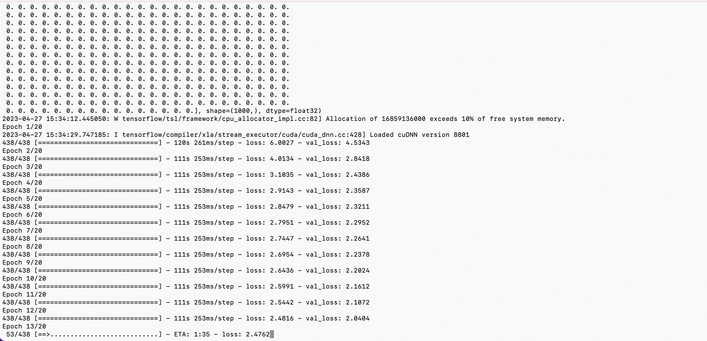
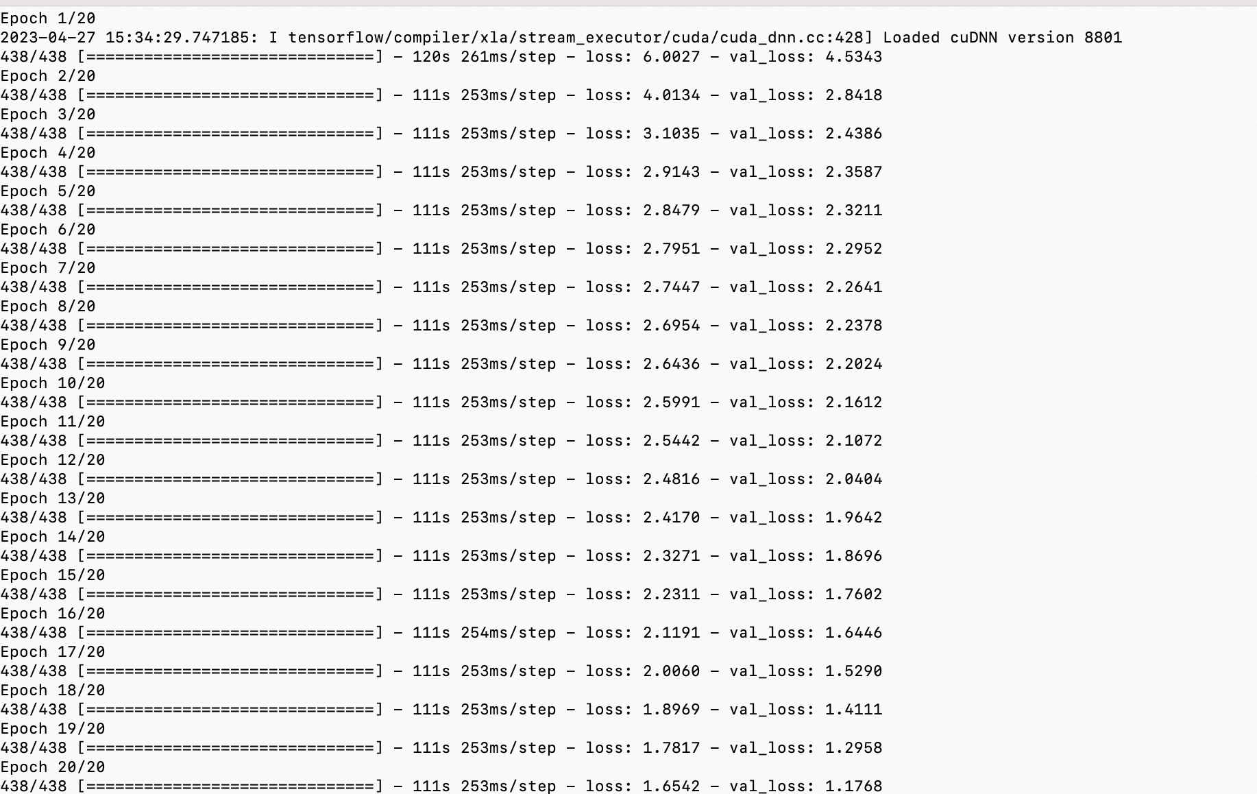
从训练过程可以看到，

即使打开了基模型的参数调整开关，fine-tune训练过程的loss收敛依然很慢，和前面章节output层10维的结构相比，收敛效果也相差了很多
由于样本集的张量维度和原始基模型output层张量维度相差较大，导致发生了过拟合的现象

增大DNN层的dropout阈值（从0.5调整到0.9），同时增加训练样本集（从50%调整到60%），尝试缓解过拟合问题，

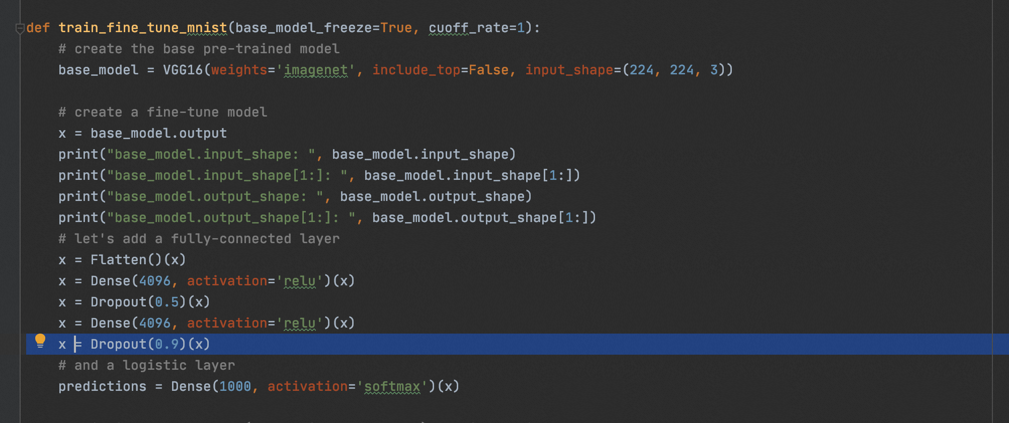
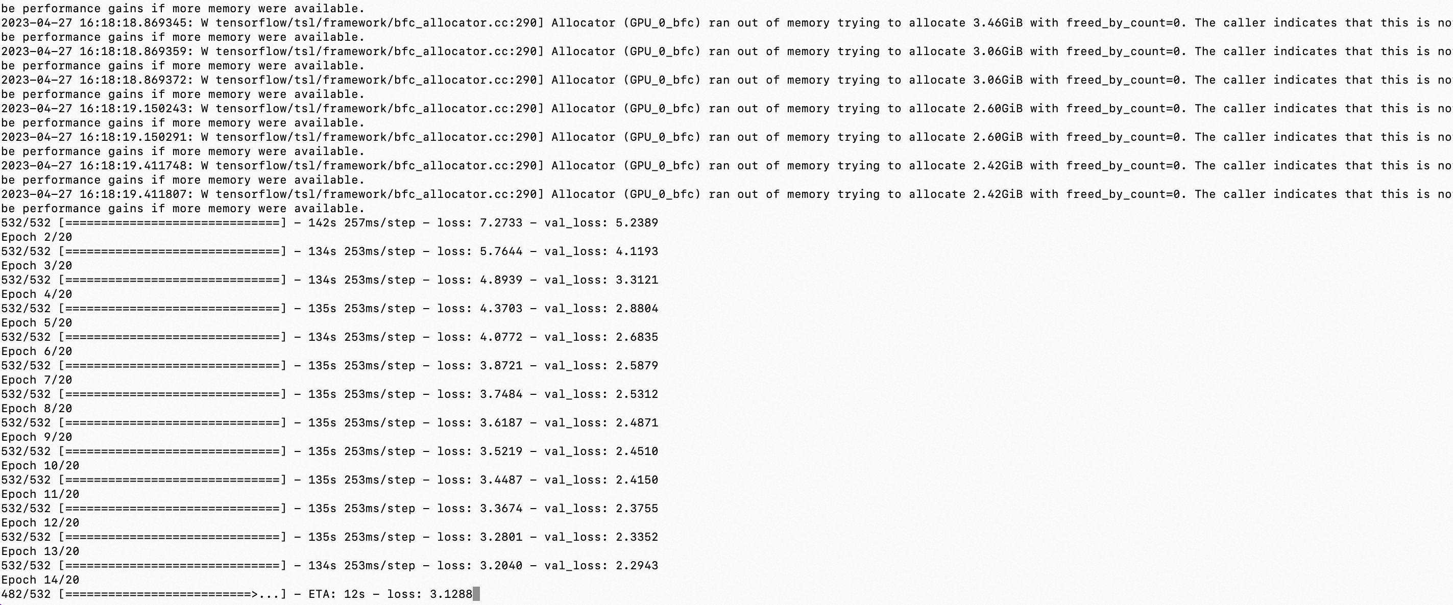
从训练过程可以看到，

即使增加了样本集，增大了正则化参数，依然无法解决过拟合问题，val_loss和loss很难收敛
因为训练集的概率空间维度（dim=10）和模型的概率预测空间维度（dim=1000）存在较大差异，因此模型被迫强行和训练集进行”对齐“，但从实验的结果来看，对齐的效果很差

使用fine-tune好的模型，对7_224.png（MNIST测试集）进行识别预测，观察迁移学习能力。

前十个图片对应的标签：　
 [7 2 1 0 4 1 4 9 5 9]

取前十张图片测试集预测：
 [1 2 1 0 1 1 1 9 3 7]

可以看到，

打开了基模型参数调整开关后，fine-tune后的模型，预测精度相比没打开开关，从20%提升到了50%
打开了基模型参数调整开关后，fine-tune后的模型，展现出了更好的能力迁移现象
因为喂入模型的新领域数据集概率空间维度，和模型的概率预测空间维度，它们之间的差异程度较大，”对齐“的效果较差

使用fine-tune好的模型，对6.webp、elephant.png进行识别预测，观察模型在旧任务上的衰退现象。

elephant.png Predicted: [[7.06066152e-12 1.82179501e-03 8.36515683e-05 4.74314615e-11
  2.22100921e-10 8.92208993e-01 4.04911802e-08 3.79545323e-04
  ....
  0.00000000e+00 0.00000000e+00 0.00000000e+00 9.86287221e-37
  1.40703496e-38 1.71527811e-36 0.00000000e+00 8.37881687e-37
  6.04951085e-37 0.00000000e+00 8.76604525e-34 0.00000000e+00]]
elephant.png Predicted: [5]


6.webp Predicted: [[1.81245338e-02 1.55029409e-06 2.25268632e-01 1.64105280e-04
  1.80434885e-08 2.65696199e-05 9.85660954e-05 7.02033997e-01
  3.46206299e-08 5.42818718e-02 0.00000000e+00 5.67526606e-35
  ...
  2.46784679e-35 1.71397608e-38 0.00000000e+00 0.00000000e+00
  0.00000000e+00 0.00000000e+00 1.02243715e-35 0.00000000e+00]]
6.webp Predicted: [7]

可以看到，

打开了基模型参数调整开关后，fine-tune后的模型，模型展现出了明显的能力衰退现象
喂入模型的新领域任务数据，和原领域任务数据的相差较大，也加剧了模型的能力衰退现象

可视化fine-tune后的基模型的卷积层，观察卷积层发生了什么变化。

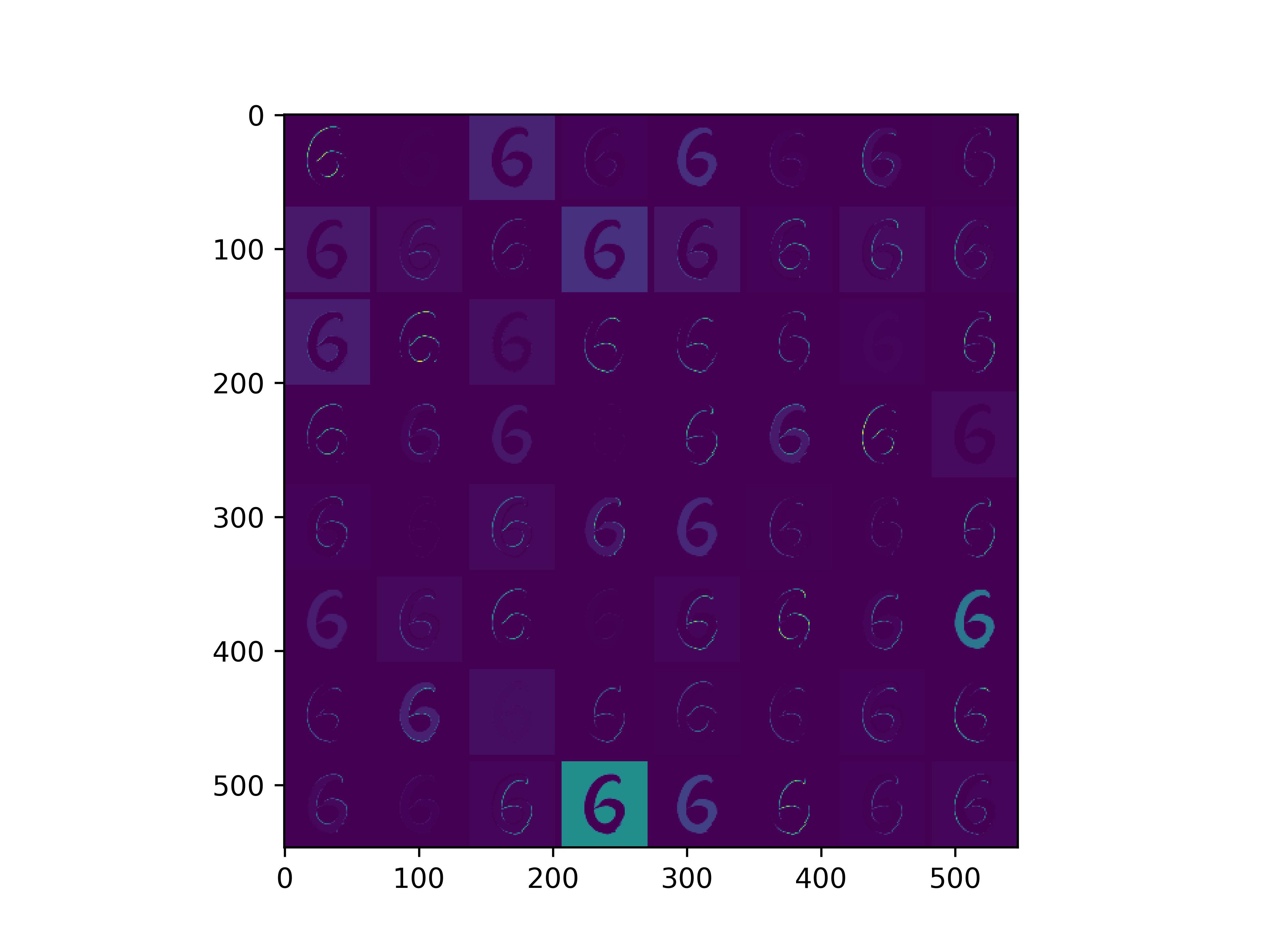
conv_block1_conv1

conv_block1_conv2

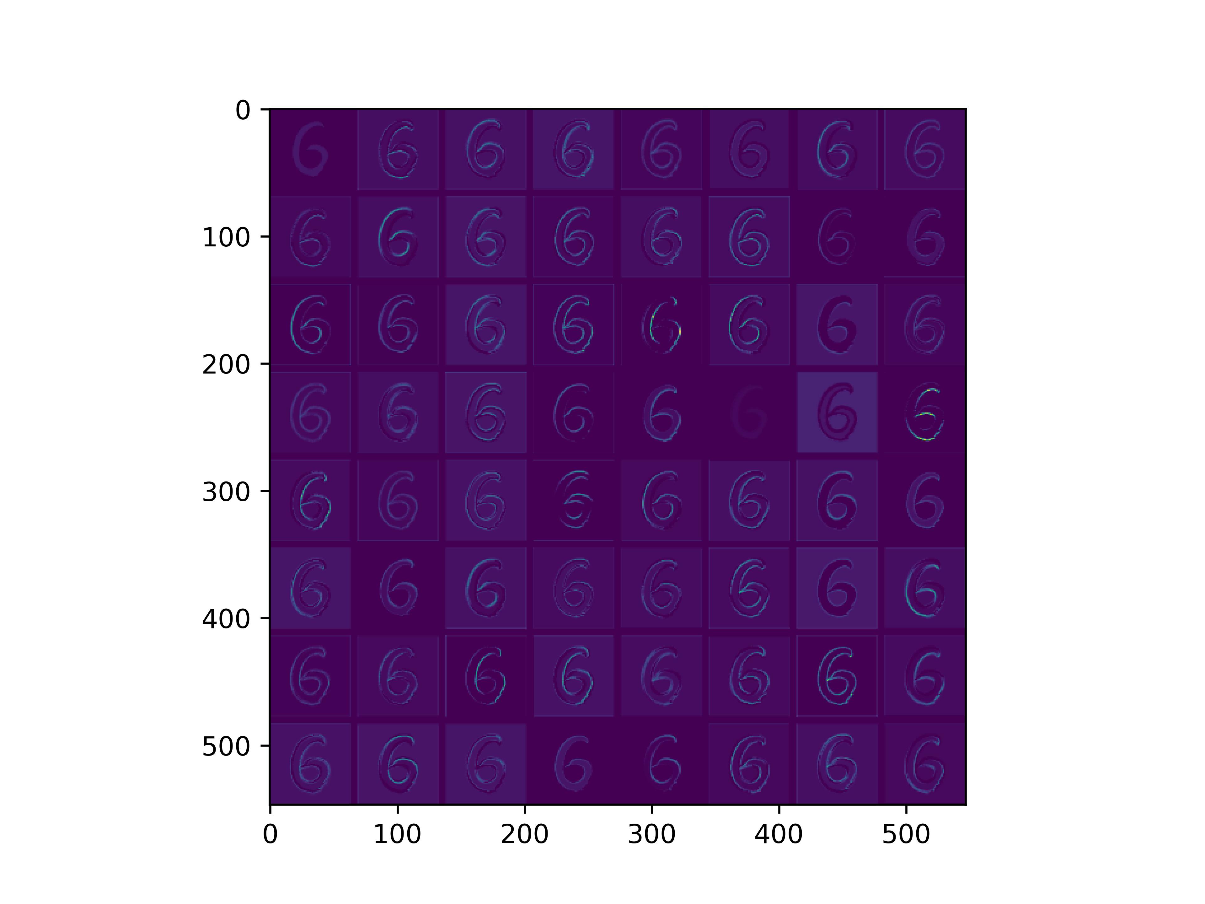
conv_block2_conv1

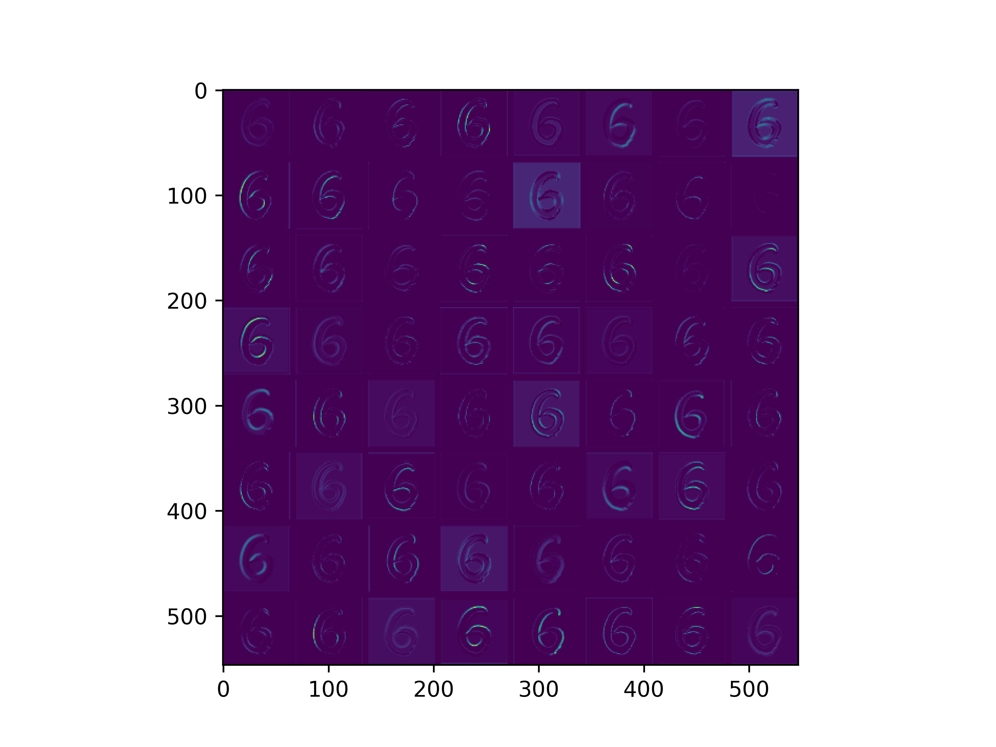
conv_block2_conv2

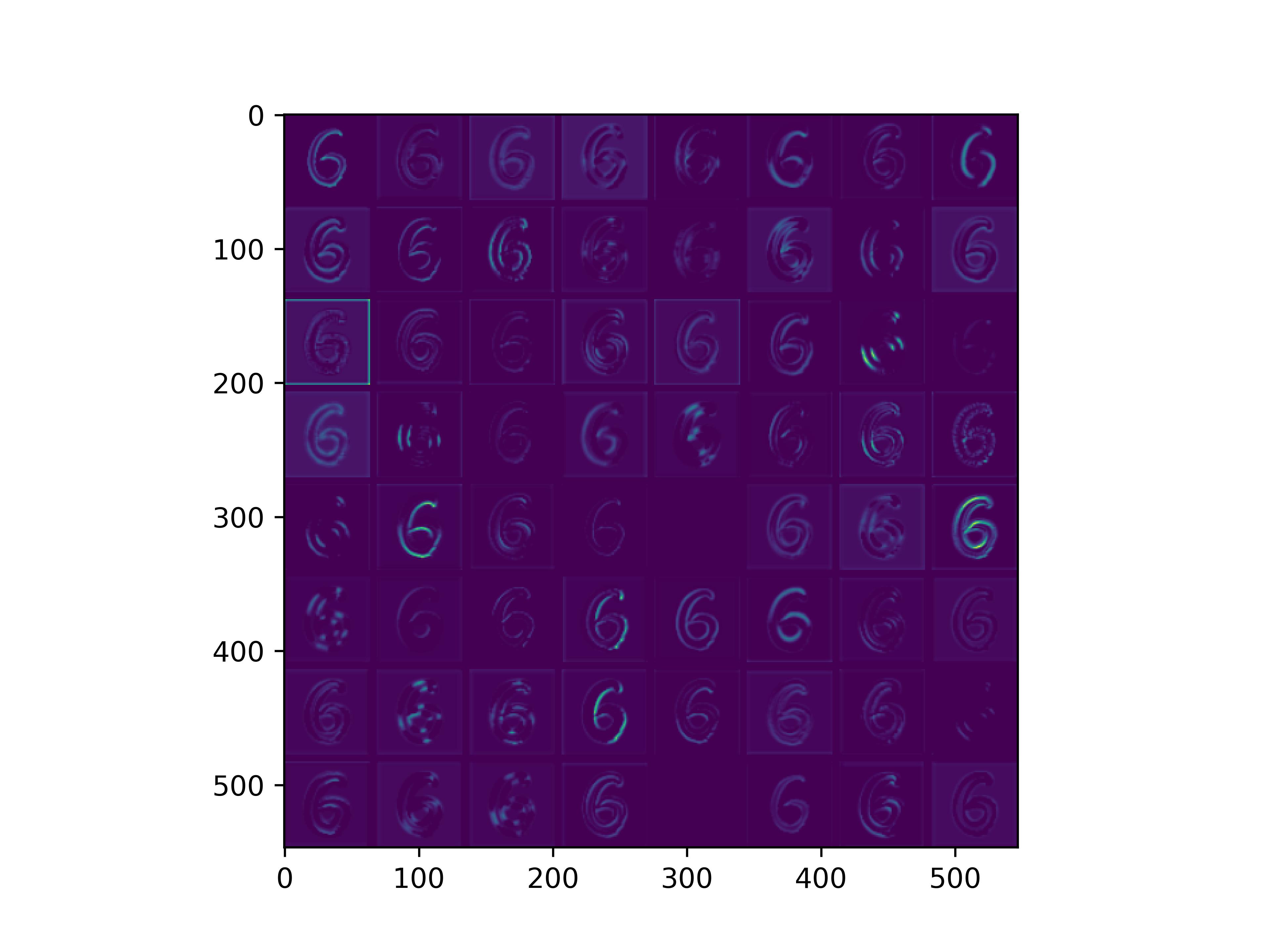
conv_block3_conv1

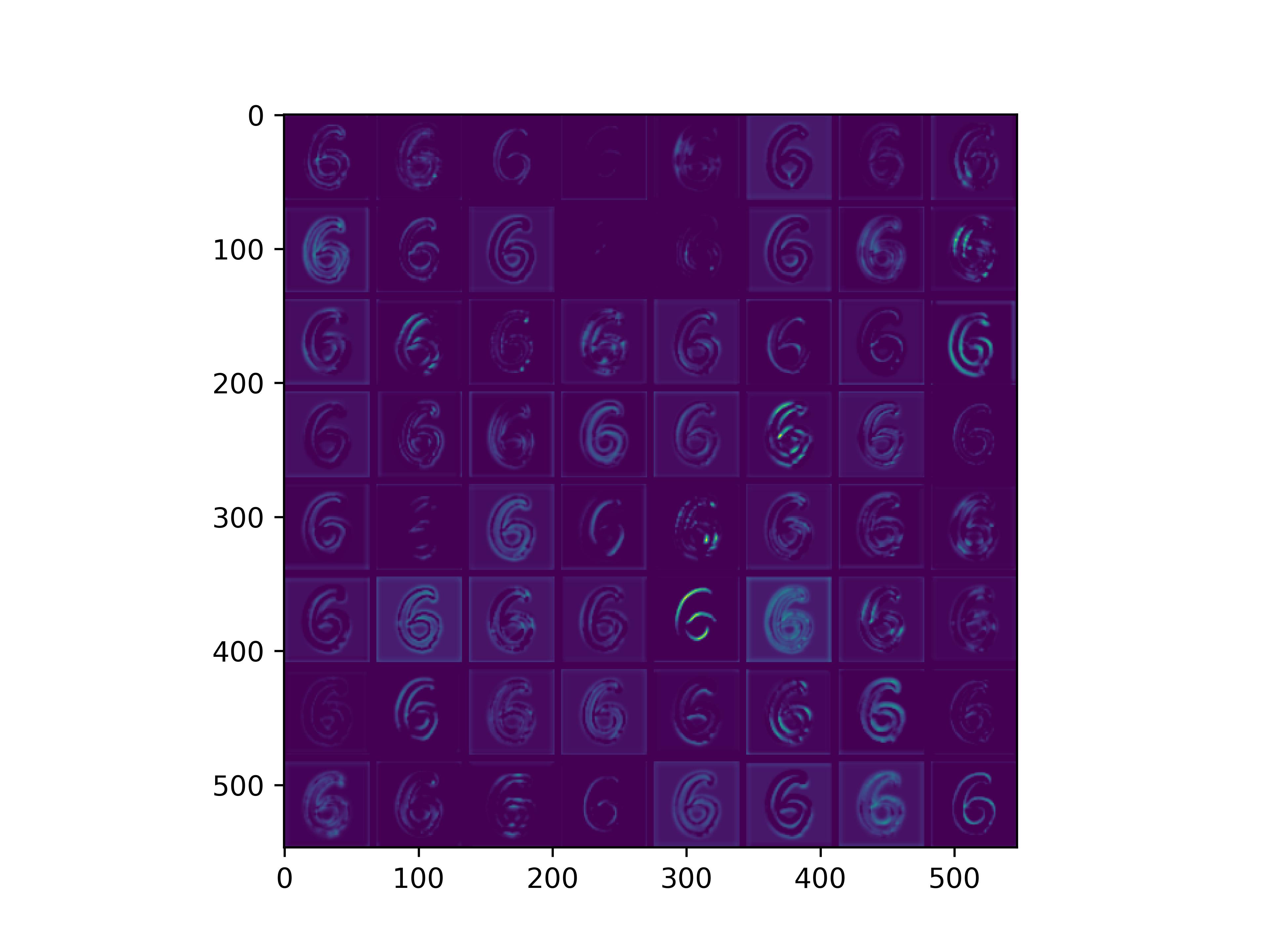
conv_block3_conv2

conv_block5_conv3

从卷积层可视化结果中可以看到，

打开了基模型参数调整开关后，基模型的卷积层感知野权重已经完成了”最优调整“（读者朋友可以和前面output dim=10的实验中可视化的卷积层相比）
即使基模新的卷积层已经提供了识别MNIST手写数字的”先验知识“，但是因为stacking后接的神经网络存在过拟和/概率预测空间维度不匹配等问题，因此最后的预测效果不好，整体上看能力迁移效果不好

0x4：实验四：在预训练基模型的基础上，基模型参数允许调整，stacking一个新的下游模型，不改变输入层和输出层的张量维度。输入MNIST手写数字图片样本（和VGG16使用的Imagenet1000存在相似但也有不同的地方）进行fine-tune训练，通过加大样本量，探寻该条件下fine-tune模型对新领域任务的迁移能力以及对原始任务的衰退现象

GPU内存OOM，待解决

0x5：实验五：设计一个dim=10中间维度的DNN stacking下游模型，并允许基模型参数调整

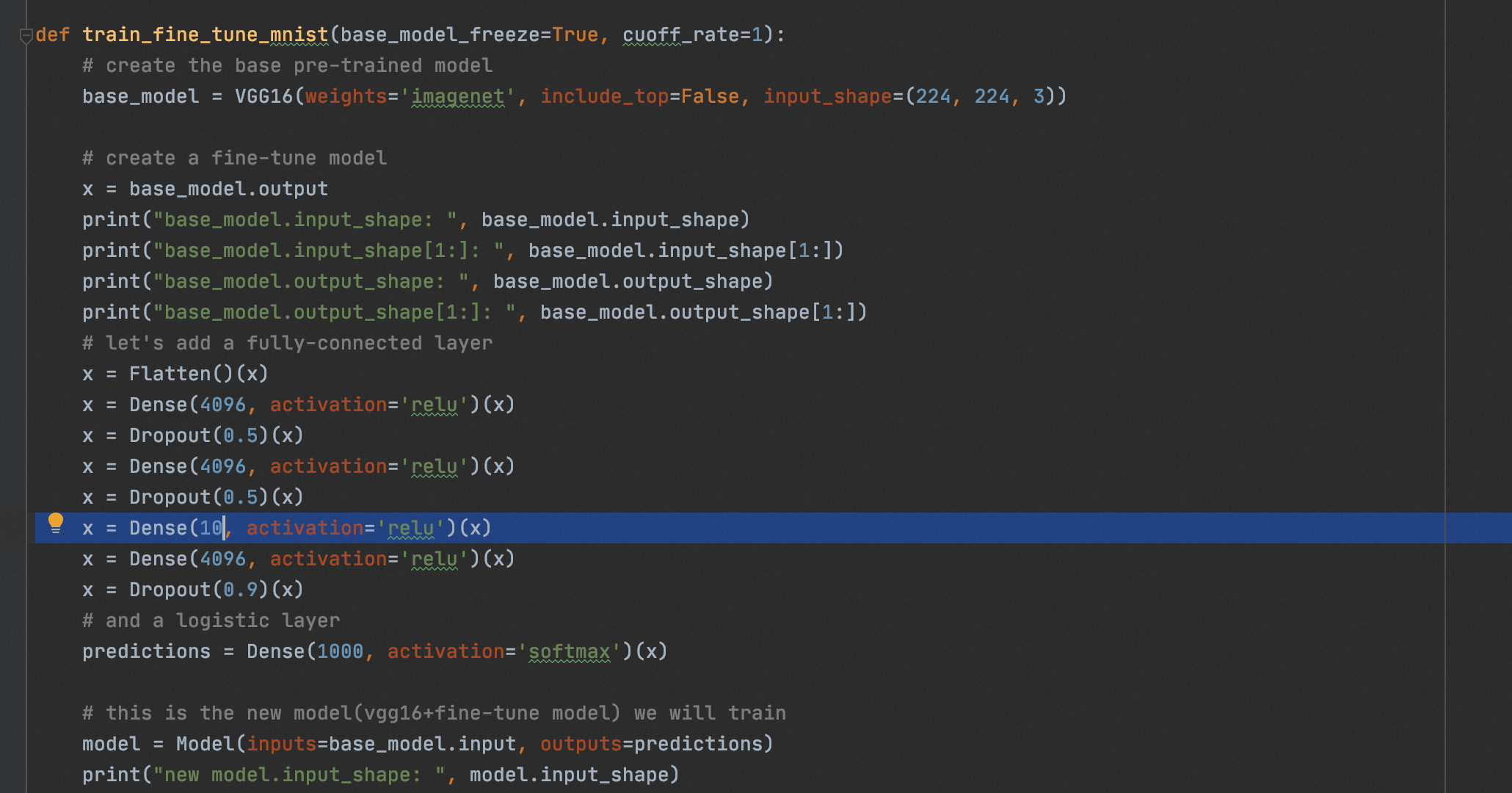
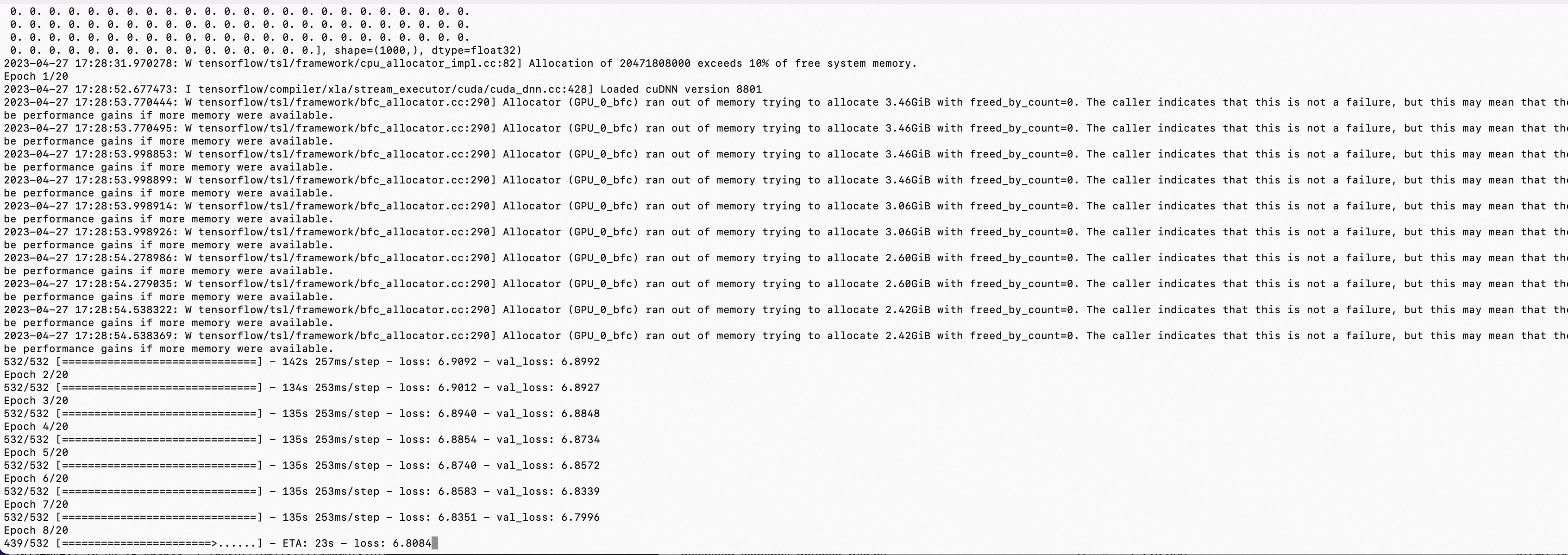
从训练过程可以看到，

一个很有趣的点，即使stacking的DNN中存在一个dim=10的fc层，理论上这一层是有机会通过训练成为一个”正确答案提供层“，但是由于这个dim=10的fc层后接了1000维的fc层，最终从整体上看，模型依然存在过拟和现象
甚至因为整体模型变复杂了，参数空间变大了，导致过拟和现象更加严重了

0x6：实验六：减小DNN stacking下游模型的复杂度和参数，并允许基模型参数调整

减少下游stacking神经网络的全连接层，

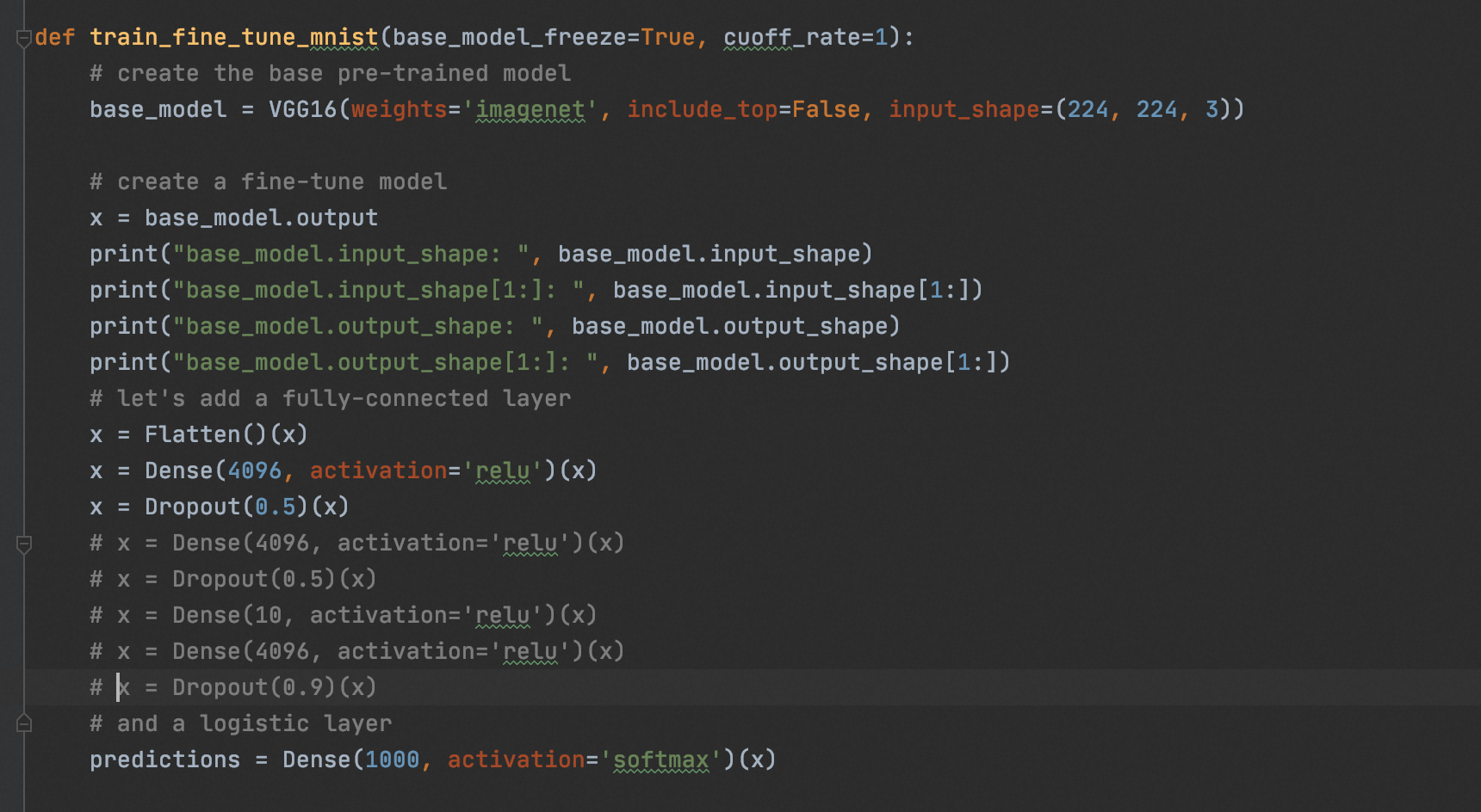
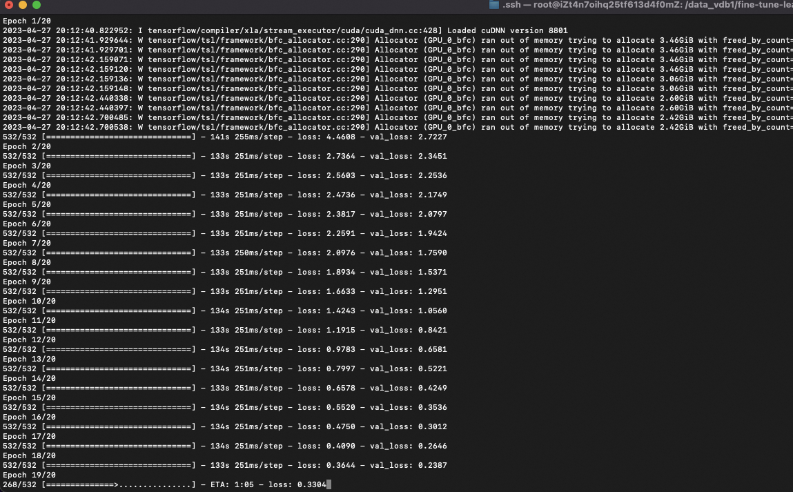
从训练过程可以看到，

通过简化下游模型结构，过拟和问题有了极大地缓解
当上游基模型已经具备下游新任务的”基础能力“的时候，下游stacking的神经网络结构不需要太复杂，通过简单的fine-tune就可以实现能力迁移

使用fine-tune好的模型，对7_224.png（MNIST测试集）进行识别预测，观察迁移学习能力。

前十个图片对应的标签：　
 [7 2 1 0 4 1 4 9 5 9]

取前十张图片测试集预测：
 [7 2 1 0 4 1 4 9 5 9]

可以看到，

通过简化下游模型结构，fine-tune后的模型，预测精度达到了100%，即实现了完美地能力迁移
即使输入模型的新领域数据集概率空间维度，和基模型的概率预测空间维度，它们之间的差异程度较大，但因为下游模型结构简单，降低了”对齐“的难度

使用fine-tune好的模型，对6.webp、elephant.png进行识别预测，观察模型在旧任务上的衰退现象。

6.webp Predicted: [547]
6.webp Predicted: [('n03272562', 'electric_locomotive', 1.0), ('n01491361', 'tiger_shark', 3.050643e-08), ('n02108915', 'French_bulldog', 2.3473039e-08)]

elephant.png Predicted: [88]
elephant.png Predicted: [('n01818515', 'macaw', 0.9995777), ('n01443537', 'goldfish', 0.00041777242), ('n02105641', 'Old_English_sheepdog', 3.08575e-06)]

可以看到，

当发生能力迁移现象时，模型对基模型原来的任务不可避免会发生能力衰退现象

0x7：实验七：减小DNN stacking下游模型的复杂度和参数，并允许基模型参数调整

四、到目前为止的发现总结

0x1：影响fine-tune效果的关键因素

基模型通过模型结构和模型参数，完成了对预训练集的”知识存储“和”知识压缩“，基模型的效果完全取决于训练样本集的范围和丰富度，在小模型上无法观测到”知识推理“、”知识涌现“等现象
基模型在stacking下游模型，喂入新领域的样本数据集，完成fine-tune后，模型对原始领域任务的处理能力会产生”能力衰退“现象，衰退的程度和几个因素有关
- 喂入模型的新领域任务数据，和原领域任务数据的相差程度，推测和数据集本身的正交相关性有关
- fine-tune过程是否freeze基模型的参数，基模型参数调整允许的范围越大，模型衰退的现象就越明显
基模型在stacking下游模型，喂入新领域的样本数据集，完成fine-tune后，模型对新领域任务会产生”能力迁移“现象，迁移的效果和几个因素有关
- 新领域任务数据，和原领域任务数据的相似程度
- fine-tune过程是否freeze基模型的参数，基模型参数调整允许的范围越大，迁移学习的效果就越好
- 喂入模型的新领域数据集概率空间维度，和模型的概率预测空间维度，它们之间的差异程度越大，”对齐“的效果就越差
- 用于fine-tune的训练集数量和丰富度（影响因素较小）
”能力迁移“和”能力衰退“是此消彼长的关系，换句话说，”能力迁移“的代价是通过”能力衰退“换取的
大模型+小模型才能产生知识迁移，即预训练模型的参数规则是关键因素，理论上，如果预训练模型足够大，能够包含下游任务的一部分核心部分，则预训练模型可以通过权重重调整，在fine-tune的过程中，激活一部分神经元以及关闭一部分神经元，以此使预训练模型朝着下游任务的方向去“生长”
下游小模型之所以仅靠少量instructions样本就可以完成迁移学习，很大程度上是因为预训练模型使用的语料库足够大和种类丰富。因为这决定了预训练模型是否完成了足够的预训练，否则如果上游预训练模型没有完成收敛，接入下游fine-tune的时候，预训练模型也依然需要进行大量的微调，这对极大拖慢整体模型的收敛。反之，如果预训练模型已经基本完成了收敛，则对下游fine-tune训练的数据集要求就很小，fine-tune就可以基于一个小数据集依然可以得到较好的效果，同时也仅需要较少的训练时间。
迁移学习也存在领域限制，预训练模型的向量化方式、张量维度、嵌入方式、编码方位、shape维度等等，和下游fine-tune任务的这些参数结构是否完全一致（或者是否具备一定的迁移性），这里的一致有两方面含义，
- 输入层的一致，理论上说，输入层的结构是一种特征工程的经验形式，它本身也代表了模型对目标任务的某种抽象。打个比方，用于文本生成任务的模型，如果将一个像素图片“强行转换适配”输入进去，最终训练和预测的效果都不好
- 输出层的一致，输出层的张量维度代表了模型的预测空间，比如一个输出层10维的模型和输出层1000维的模型，它们之间就不具备迁移条件。打个比方，用一个1000类物体识别的模型去做10类数字识别，最终的预测效果就不好，因为这很容易导致模型过拟合

0x2：改进fine-tune效果以及提升领域应用的可行方向

1、大模型开发、优化、理论分析方向 - model dev

【train from scratch】收集、清洗、整理更多不同领域的高质量数据集，扩大基模型训练样本量，增加基模型的知识存储密度，基模型更大的知识密度，意味着和下游任务有更高概率存在相似性，也即同时更容易在fine-tune后产生能力迁移
【more model scale】在计算架构、成本等可控的前提下，优化大模型神经网络结构，提高基模型参数规模

更大的规模可以存储更多的知识，并有机会产生知识推理和涌现现象
更优化的神经网络结构可以更有效地提取语料知识，有助于能力迁移的效果

【optimizing the stacking structure】研究、开发、设计更优的基模型stacking结构（例如适配二分类、多分类等任务的stacking结构），改进现有prompt-tune、prefix-tune、p-tune、lora微调算法，探索更优的基模型参数微调算法，以帮助下游任务更好地完成能力迁移

2、业务场景定制开发、应用方向 - model train

在计算架构、成本等可控的前提下，在fine-tune时打开基模型的参数调整，以获取更好的能力迁移效果
在设计fine-tune train dataset template的时候，要注意新旧任务在概率预测空间上的差异，以获取更好的能力迁移效果。输入样本维度/输出的概率预测空间，要和基模型的输入和输出结构保持基本一致或近似一致，否则强行fine-tune会出现过拟合问题，
- 列举几个典型的不适应场景
  - 用output概率预测空间1000dim的图像识别大模型，fine-tune一个output概率预测空间10dim的图像识别任务
  - 用output概率预测空间13Bdim的文本生成大模型，fine-tune一个output概率预测空间2dim的二分类文本分类任务，输入N个 Ndim token/输入1个 2dim token
- 列举几个典型的适用场景
  - 用output概率预测空间1000dim的图像识别大模型，fine-tune一个output概率预测空间10dim的图像识别任务（识别的类型可能不一样）
  - 用output概率预测空间13Bdim的文本生成大模型，fine-tune一个output概率预测空间10000dim的文本生成任务，输入N个 Ndim token/输入N个 10000dim token
在基模型足够好的前提下，fine-tune的数据集数量的重要性相对减弱了，这会极大降低大模型在各个领域的应用难度和应用门槛
在基模型参数规模、参数收敛性、参数丰富度等性能足够强的前提下，下游模型仅需要相对简单的结构就可以产生能力迁移，并不要特别复杂的模型结构，这对fine-tune任务的计算开销相对会较小

3、基于内外部开源大模型优化fewshot prompt应用效果方向 - model predict

根据下游任务的具体领域要求和安全攻防知识，设计、优化fewshot prompt template，引导模型更多地生成业务需求的语料文本

4、数据标注

根据安全不同领域具体需求，对原始数据进行人工标注、prompt生成（input-output格式）等任务
- 根据一段恶意代码，生成对应的prompt提示
- ...
根据特定的任务（例如免杀shellcode生成、恶意代码生成等），人工进行逐步prompt优化，记录整个prompt引导过程，生成的prompt引导日志可以用于后续的强化学习

posted @ 2023-04-26 17:51 郑瀚Andrew 阅读(2621) 评论(0) 编辑收藏举报

会员力量，点亮园子希望

刷新页面返回顶部

Han Zheng, Practitioners and Theoretical Researcher, Now working in Alibaba Cloud Corp, China

Welcome to contact me. Wechat：LittleHann，My email, 306211321@qq.com，Job mail：zhenghan.zh@alibaba-inc.com

深度学习网络微调（fine-tune）的基本原理以及应用约束条件 - 以VGG卷积神经网络迁移学习MNIST手写识别任务为例进行的一些实验和总结发现

一、模型预训练通俗理解

0x1：什么是预训练模型（pre-trained model）

0x2：什么是模型微调

0x3：为什么要微调？

0x4：不同数据集下如何进行微调

1、数据量少，但数据相似度非常高

2、数据量少，数据相似度低

3、数据量大，数据相似度低

4、数据量大，数据相似度高

0x5：微调指导事项

二、通过卷积核可视化探究fine-tune本质

0x1：直接基于VGG16进行手写数字预测

0x2：通过手写数字，可视化VGG16各个层参数

0x3：使用VGG16作为预训练模型，fine-tune一个手写数字识别卷积网络，再观察基模型和fine-tune模型的可视化

1、直接设计一个CNN卷积网络进行手写数字识别

2、冻结预训练基模型，调整下游fine-tune层参数：VGG16 without toplayer + 全连接层 迁移学习

3、允许预训练基模型参数微调，同时调整下游fine-tune层参数：VGG16 without toplayer + 全连接层 迁移学习

0x4：用于下游任务的样本量大小对fine-tune效果的影响

1、cutoff rate=90% MNIST手写数字识别样本、50epoch - 高质量、海量样本、多轮训练

2、cutoff rate=50% MNIST手写数字识别样本、50epoch - 高质量、中等数量样本

3、cutoff rate=10% MNIST手写数字识别样本、50epoch - 高质量、较少样本

4、cutoff rate=2.5% MNIST手写数字识别样本、50epoch - 高质量、少量样本

5、cutoff rate=2.5% MNIST手写数字识别样本、1000epoch - 高质量、少量样本、超多轮次训练

6、cutoff rate=1% MNIST手写数字识别样本、2000epoch - 高质量、极少量样本、超多轮次训练

7、cutoff rate=0.5% MNIST手写数字识别样本、2000epoch - 高质量、极少量样本、超多轮次训练

8、cutoff rate=0.25% MNIST手写数字识别样本、5000epoch - 高质量、极少量样本、超多轮次训练、更小batchsize、更慢学习速率

9、cutoff rate=0.35% MNIST手写数字识别样本、5000epoch - 高质量、极少量样本（轻微加大样本量）、超多轮次训练

10、cutoff rate=0.25% MNIST手写数字识别样本、5000epoch - 高质量、极少量样本（样本量不变）、超多轮次训练、（继续降低学习率和batchsize）

结论总结：

三、通过VGG16迁移学习探寻基模型fine-tune/训练级驱动对齐技术的基本原理和应用边界条件

0x1：实验一：可视化VGG16各层卷积层

0x5：实验五：设计一个dim=10中间维度的DNN stacking下游模型，并允许基模型参数调整

0x6：实验六：减小DNN stacking下游模型的复杂度和参数，并允许基模型参数调整

0x7：实验七：减小DNN stacking下游模型的复杂度和参数，并允许基模型参数调整

四、到目前为止的发现总结

0x1：影响fine-tune效果的关键因素

0x2：改进fine-tune效果以及提升领域应用的可行方向

1、大模型开发、优化、理论分析方向 - model dev

2、业务场景定制开发、应用方向 - model train

3、基于内外部开源大模型优化fewshot prompt应用效果方向 - model predict

4、数据标注

公告

2、冻结预训练基模型，调整下游fine-tune层参数：VGG16 without toplayer + 全连接层迁移学习

3、允许预训练基模型参数微调，同时调整下游fine-tune层参数：VGG16 without toplayer + 全连接层迁移学习