用AutoEncoder做一些有趣的事情
用AutoEncoder做一些有趣的事情
有人甚至做了Mask AutoEncoder之类的东西,第一次知道可以这样去恢复原数据,真的非常有意思。可以在这里也试一下AutoEncoder,下面用了mnist俩个数据集(一个最经典的、一个FashionMnist,只需要切换一下datasets那里的数据运行便可以看到效果)。
- 本笔记特意投影到三维的区间方便用三维空间画出十种数据在autoEncoder降维之后十如何分布的,我们通过三维图看到相同的数据还是分布在一块,也就是说明了降维成功了。而且这些数据也能很好的刻画原数据的值(最后的测试集可以看到效果)。
- 最后利用测试集的数据进行随机的图片生成,这里的应用我们可能以后会想到token的应用,提取关键词,用decoder生成图片(对应之后的diffusion模型)
- 我们线性地去改变三维向量的值看一下生成的图像结果变化
加入库
# Import PyTorch modules
import torch
import torch.nn as nn
import torch.optim as optim
import torchvision.datasets as datasets
import torchvision.transforms as transforms
# 打印torch和torchvision的版本
import torchvision
print(torch.__version__)
print(torchvision.__version__)
1.13.1+cu116
0.14.1+cu116
查看显卡资源
!nvidia-smi
Wed Feb 22 15:32:52 2023
+-----------------------------------------------------------------------------+
| NVIDIA-SMI 510.47.03    Driver Version: 510.47.03    CUDA Version: 11.6     |
|-------------------------------+----------------------+----------------------+
| GPU  Name        Persistence-M| Bus-Id        Disp.A | Volatile Uncorr. ECC |
| Fan  Temp  Perf  Pwr:Usage/Cap|         Memory-Usage | GPU-Util  Compute M. |
|                               |                      |               MIG M. |
|===============================+======================+======================|
|   0  Tesla T4            Off  | 00000000:00:04.0 Off |                    0 |
| N/A   65C    P0    31W /  70W |    858MiB / 15360MiB |      0%      Default |
|                               |                      |                  N/A |
+-------------------------------+----------------------+----------------------+

+-----------------------------------------------------------------------------+
| Processes:                                                                  |
|  GPU   GI   CI        PID   Type   Process name                  GPU Memory |
|        ID   ID                                                   Usage      |
|=============================================================================|
|    0   N/A  N/A    542863      C                                     855MiB |
+-----------------------------------------------------------------------------+
定义超参数
device = torch.device('cuda' if torch.cuda.is_available() else 'cpu')
# Define hyperparameters
batch_size = 100
num_epochs = 20
learning_rate = 0.001
加载数据集
数据集我们使用了用了两个数据集,发现效果均很好,要切换的话把下面的注释 切换注释即可,下面展示的结果都是在FashionMNIST上的;
# Load MNIST dataset
# train_dataset = datasets.MNIST(root='data/', train=True, transform=transforms.ToTensor(), download=True)
# test_dataset = datasets.MNIST(root='data/', train=False, transform=transforms.ToTensor(), download=True)
train_dataset = datasets.FashionMNIST(root='data/', train=True, transform=transforms.ToTensor(), download=True)
test_dataset = datasets.FashionMNIST(root='data/', train=False, transform=transforms.ToTensor(), download=True)
train_loader = torch.utils.data.DataLoader(train_dataset, batch_size=batch_size, shuffle=True)
test_loader = torch.utils.data.DataLoader(test_dataset, batch_size=batch_size, shuffle=False)
Downloading http://fashion-mnist.s3-website.eu-central-1.amazonaws.com/train-images-idx3-ubyte.gz
Downloading http://fashion-mnist.s3-website.eu-central-1.amazonaws.com/train-images-idx3-ubyte.gz to data/FashionMNIST/raw/train-images-idx3-ubyte.gz


  0%|          | 0/26421880 [00:00<?, ?it/s]


Extracting data/FashionMNIST/raw/train-images-idx3-ubyte.gz to data/FashionMNIST/raw

Downloading http://fashion-mnist.s3-website.eu-central-1.amazonaws.com/train-labels-idx1-ubyte.gz
Downloading http://fashion-mnist.s3-website.eu-central-1.amazonaws.com/train-labels-idx1-ubyte.gz to data/FashionMNIST/raw/train-labels-idx1-ubyte.gz


  0%|          | 0/29515 [00:00<?, ?it/s]


Extracting data/FashionMNIST/raw/train-labels-idx1-ubyte.gz to data/FashionMNIST/raw

Downloading http://fashion-mnist.s3-website.eu-central-1.amazonaws.com/t10k-images-idx3-ubyte.gz
Downloading http://fashion-mnist.s3-website.eu-central-1.amazonaws.com/t10k-images-idx3-ubyte.gz to data/FashionMNIST/raw/t10k-images-idx3-ubyte.gz


  0%|          | 0/4422102 [00:00<?, ?it/s]


Extracting data/FashionMNIST/raw/t10k-images-idx3-ubyte.gz to data/FashionMNIST/raw

Downloading http://fashion-mnist.s3-website.eu-central-1.amazonaws.com/t10k-labels-idx1-ubyte.gz
Downloading http://fashion-mnist.s3-website.eu-central-1.amazonaws.com/t10k-labels-idx1-ubyte.gz to data/FashionMNIST/raw/t10k-labels-idx1-ubyte.gz


  0%|          | 0/5148 [00:00<?, ?it/s]


Extracting data/FashionMNIST/raw/t10k-labels-idx1-ubyte.gz to data/FashionMNIST/raw
查看数据集shape
print(train_dataset.data.shape)
print(test_dataset.data.shape)
torch.Size([60000, 28, 28])
torch.Size([10000, 28, 28])
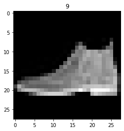
展示测试集图像
# 用plt显示一张图片
import matplotlib.pyplot as plt
plt.imshow(test_dataset.data[0].numpy(), cmap='gray')
plt.title('%i' % test_dataset.targets[0])
plt.show()
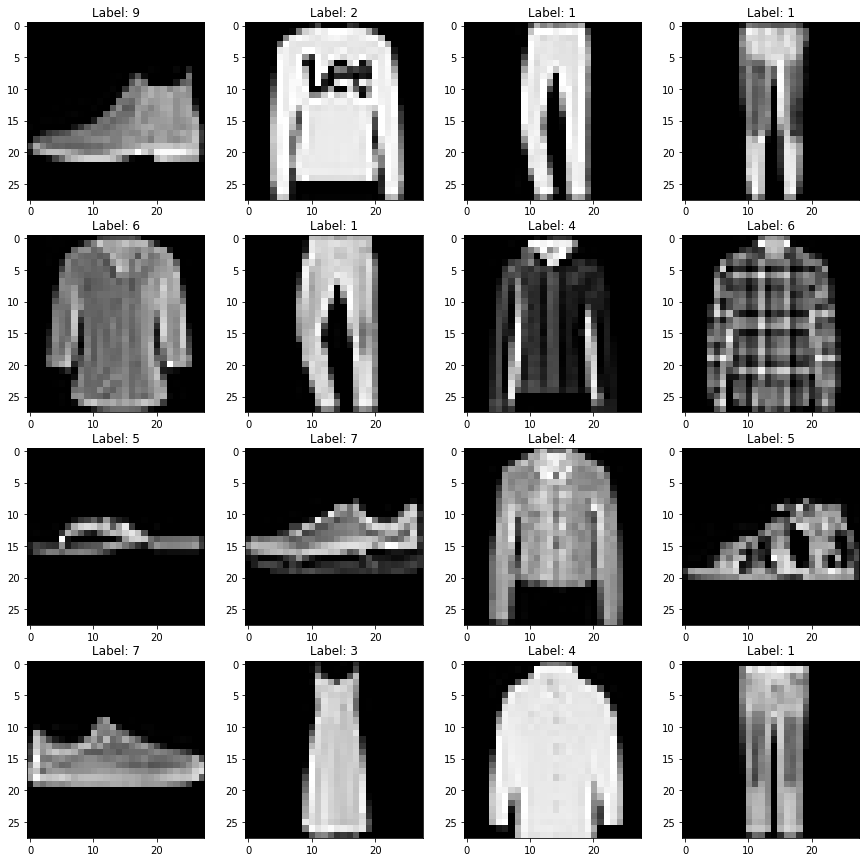
展示多张图片
# Import matplotlib.pyplot module for plotting images
import matplotlib.pyplot as plt
# Plot some sample images from test dataset
for data in test_loader:
    # Get input images and labels
    img,label  = data
    img = img.to(device)
    label = label.to(device)

    # Plot a grid of 16 images with their labels
    fig ,axs = plt.subplots(4 ,4 ,figsize=(15 ,15))
    for i in range(4):
        for j in range(4):
            # Get image tensor at index i*4+j index i*4+j image img[index]
            index = i*4+j
            image = img[index]
            # Convert image tensor to numpy array and transpose it to HxWxC format
            image = image.cpu().numpy().transpose(1 ,2 ,0)

            # Plot image on subplot
            axs[i][j].imshow(image.squeeze() ,cmap='gray')
            axs[i][j].set_title(f'Label: {label[index].item()}')
    # Show the figure
    plt.show()
    # Break after one batch
    break
定义网络
# Define autoencoder model
class Autoencoder(nn.Module):
    def __init__(self):
        super(Autoencoder, self).__init__()
        # Encoder layers
        self.encoder = nn.Sequential(
            nn.Linear(28*28, 128),
            nn.ReLU(),
            nn.Linear(128, 64),
            nn.ReLU(),
            nn.Linear(64, 12),
            nn.ReLU(),
            nn.Linear(12, 3) # Latent space representation
        )
        # Decoder layers
        self.decoder = nn.Sequential(
            nn.Linear(3, 12),
            nn.ReLU(),
            nn.Linear(12, 64),
            nn.ReLU(),
            nn.Linear(64, 128),
            nn.ReLU(),
            nn.Linear(128, 28*28),
            nn.Sigmoid() # To get values between 0 and 1 for pixel values
        )

    def forward(self, x):
        # Encode input to latent space representation
        encoded = self.encoder(x)
        # Decode latent space representation to reconstructed output
        decoded = self.decoder(encoded)
        return decoded

# Define convolutional autoencoder model: 这个使用了卷积的autoEncoder在这里没有用到,因为要对维度做一些修改,为了简洁所以没有放在这里
class ConvAutoencoder(nn.Module):
    def __init__(self):
        super(ConvAutoencoder, self).__init__()
        # Encoder layers
        self.encoder = nn.Sequential(
            nn.Conv2d(1, 16, 3, stride=2, padding=1), # (N, 1, 28, 28) -> (N, 16, 14 ,14)
            nn.ReLU(),
            nn.Conv2d(16 ,32 ,3 ,stride=2 ,padding=1), # (N ,16 ,14 ,14) -> (N ,32 ,7 ,7)
            nn.ReLU(),
            nn.Conv2d(32 ,64 ,7), # (N ,32 ,7 ,7) -> (N ,64 ,1 ,1)
        )
        # Decoder layers
        self.decoder = nn.Sequential(
            nn.ConvTranspose2d(64 ,32 ,7), # (N ,64 ,1 ,1) -> (N ,32 ,7 ,7)
            nn.ReLU(),
            nn.ConvTranspose2d(32, 16, 3,stride=2,padding=1,output_padding=1), # (N .32 .7 .7) -> (N .16 .14 .14)
            nn.ReLU(),
            nn.ConvTranspose2d(16, 1, 3,stride=2,padding=1,output_padding=1), # (N .16 .14 .14) -> (N .1 .28 .28)
            nn.Sigmoid() # To get values between 0 and 1 for pixel values
        )

    def forward(self,x):
        # Encode input to latent space representation
        encoded = self.encoder(x)
        # Decode latent space representation to reconstructed output
        decoded = self.decoder(encoded)
        return decoded
模型定义
# Create model instance and move it to device (GPU or CPU)
model = Autoencoder()
# model = ConvAutoencoder()
device = torch.device("cuda" if torch.cuda.is_available() else "cpu")
model.to(device)


# Define loss function and optimizer
criterion = nn.MSELoss(reduction = 'none') # Mean Squared Error loss for reconstruction error
optimizer = optim.Adam(model.parameters(), lr=learning_rate)
开始训练并评估
print(len(train_loader.dataset))
print(len(test_loader.dataset))
60000
10000
train_loader.dataset为调用原dataset的一个方法,由于len(train_loader)的大小可能是不固定的:比如batch_size为64的话,训练集上(60000个样本)就一定会有一个batch是32个样本(\(60000 \% 64 = 32\)),测试集上也会有一个batch是16个样本(\(10000 \% 64 = 16\)),虽然大多数样本都是设定好的64,不过肯定有一个batch的样本是剩下不够的(除非我们选取的batch刚刚好)。
train_loss_list = [] # To store training loss for each epoch
test_loss_list = [] # To store test loss for each epoch
# Training loop
for epoch in range(num_epochs):
    train_loss = 0
    test_loss = 0
    train_example_num = 0
    test_example_num = 0

    # =================== Testing ===================
    model.eval() # Set model to evaluation mode
    with torch.no_grad(): # Disable gradient calculation
        for data in test_loader:
            # Get input images and flatten them to vectors of size 784 (28*28)
            img, _ = data
            img = img.view(img.size(0), -1)
            img = img.to(device)

            # Forward pass to get reconstructed output
            output = model(img)

            # Compute reconstruction loss
            loss = criterion(output, img)
            loss = loss.mean()

            test_loss += loss.item() * img.size(0)
            test_example_num += img.size(0)


    # =================== Training ===================
    model.train() # Set model to training mode
    for data in train_loader:
        # Get input images and flatten them to vectors of size 784 (28*28)
        img, _ = data
        img = img.to(device)
        img = img.view(img.size(0), -1)


        # Forward pass to get reconstructed output
        output = model(img)

        # Compute reconstruction loss
        loss = criterion(output, img)
        loss = loss.mean()

        # Backward pass and update parameters
        optimizer.zero_grad()
        loss.backward()
        optimizer.step()

        train_loss += loss.item() * img.size(0)
        train_example_num += img.size(0)


    # =================== Logging ===================
    # Save training loss
    train_loss_list.append(train_loss/60000) # train_loader.dataset is the entire dataset
    # Save test loss
    test_loss_list.append(test_loss/10000) # test_loader.dataset is the entire dataset

    # Print training and test loss for each epoch
    print(f"Epoch {epoch+1}/{num_epochs}, Train Loss: {train_loss_list[-1]:.4f}, Test Loss: {test_loss_list[-1]:.4f}")
Epoch 1/20, Train Loss: 0.0505, Test Loss: 0.1701
Epoch 2/20, Train Loss: 0.0339, Test Loss: 0.0364
Epoch 3/20, Train Loss: 0.0282, Test Loss: 0.0302
Epoch 4/20, Train Loss: 0.0264, Test Loss: 0.0269
Epoch 5/20, Train Loss: 0.0256, Test Loss: 0.0260
Epoch 6/20, Train Loss: 0.0252, Test Loss: 0.0255
Epoch 7/20, Train Loss: 0.0248, Test Loss: 0.0250
Epoch 8/20, Train Loss: 0.0244, Test Loss: 0.0249
Epoch 9/20, Train Loss: 0.0241, Test Loss: 0.0244
Epoch 10/20, Train Loss: 0.0238, Test Loss: 0.0242
Epoch 11/20, Train Loss: 0.0235, Test Loss: 0.0237
Epoch 12/20, Train Loss: 0.0232, Test Loss: 0.0235
Epoch 13/20, Train Loss: 0.0230, Test Loss: 0.0236
Epoch 14/20, Train Loss: 0.0228, Test Loss: 0.0231
Epoch 15/20, Train Loss: 0.0227, Test Loss: 0.0230
Epoch 16/20, Train Loss: 0.0225, Test Loss: 0.0230
Epoch 17/20, Train Loss: 0.0224, Test Loss: 0.0226
Epoch 18/20, Train Loss: 0.0223, Test Loss: 0.0226
Epoch 19/20, Train Loss: 0.0222, Test Loss: 0.0225
Epoch 20/20, Train Loss: 0.0221, Test Loss: 0.0226
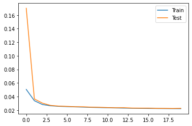
画出train_loss和test_loss的曲线图
上面我们定义的train_loss和test_loss都是指单个样本的损失值(平均损失),也可以注意到里面每个epoch里面我们都是先算的test_loss再算的train_loss,因为这样才能使得test_loss是一直高于train_loss的正常结果(我们不能先算train_loss再利用梯度下降好的网络去求test_loss,因为求loss的时候肯定是要求网络的参数是不变的、无论针对的是训练集还是测试集)
# Plot training and test loss
plt.plot(train_loss_list, label="Train")
plt.plot(test_loss_list, label="Test")
plt.legend()
plt.show()
看一下encoder的结果
查看单个样本的encoder之后的结果
data_tmp = test_dataset.data[0].view(-1)
data_tmp.shape
torch.Size([784])
data_tmp.dtype
torch.uint8
data_tmp = data_tmp.float().to(device)
test_dataset.data.view(10000,-1).shape
torch.Size([10000, 784])
with torch.no_grad():
  output = model.encoder(data_tmp)
output
tensor([-1947.6212, 793.4739, 1010.8380], device='cuda:0')
求整个测试集encoder之后的结果
# 得到encoded 测试集
model.eval() # Set model to evaluation mode
with torch.no_grad(): # Disable gradient calculation
    # Get input images and flatten them to vectors of size 784 (28*28)
    img = test_dataset.data
    img = img.view(10000,-1)
    img = img.float().to(device)

    # Forward pass to get reconstructed output
    output = model.encoder(img)
    test_encoded = output.cpu().numpy()
test_encoded.shape
(10000, 3)
test_encoded[0]
array([-440.385 , 887.1012 , 338.86945], dtype=float32)
画出三维图
# 用Axes3D画3d图
from mpl_toolkits.mplot3d import Axes3D

# 画3d图,标签为test_dataset.targets
fig = plt.figure()
ax = Axes3D(fig)
ax.scatter(test_encoded[:,0], test_encoded[:,1], test_encoded[:,2], c=test_dataset.targets)
plt.show()
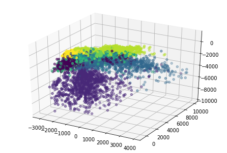
在上面代码的开头加入%matplotlib notebook还可以使得交互变为动态的形式,不过在vscode或者colab这种笔记本下是加载不出来的,只有jupyter notebook才行,可以看到很好测试集的\(28\times28\)投影到\(\R^{3}\)之后的每个点都被很好的分散开来了,而且相同类比的点都在空间中比较近的地方(实际上我们点一开始应该是都处于三维坐标系中的一个位置,在网络的训练之后所有点就都被推到自己应该在的位置了——也就是梯度下降)
.assets/mnist三维编码图.gif)
保存数据
import numpy as np
import matplotlib.pyplot as plt
# 保存 test_encoded 为 test_encoded.csv
np.savetxt('test_encoded_fashionMnist.csv', test_encoded, delimiter = ',')

# 保存 test_dataset.targets 为 test_dataset_targets.csv
np.savetxt('test_dataset_targets_fashionMnist.csv', test_dataset.targets, delimiter = ',')
查看测试集效果
test_encoded[3]
array([ -652.92444, 1792.8131 , -4744.6997 ], dtype=float32)
求测试集上的均值和方差
mean = test_encoded.mean(axis=0)
std = test_encoded.std(axis=0)
print("mean", mean)
print("std", std)
mean [ -711.3988  2512.099  -1240.0192]
std [ 979.6909 1675.2717 1836.2504]
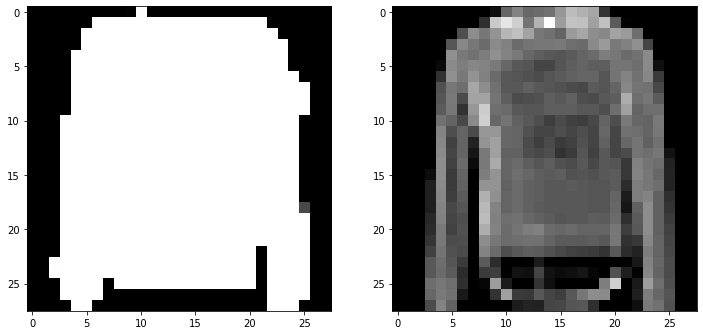
展示测试集上生成图片和正确结果图像
# rand_np = np.random.rand(1,3)*std + mean
idx = 16
rand_np = test_encoded[idx]
tensor = torch.from_numpy(rand_np).float().to(device)

# 得到encoded 测试集
model.eval() # Set model to evaluation mode
with torch.no_grad(): # Disable gradient calculation
    # Forward pass to get reconstructed output
    img = model.decoder(tensor)
    img_np = img.cpu().numpy()

plt.figure(figsize=(12,8))
plt.subplot(1,2,1)
plt.imshow(img_np.reshape(28,28), cmap='gray')
plt.subplot(1,2,2)
plt.imshow(test_dataset.data[idx], cmap='gray')
plt.show()
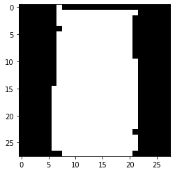
用三维坐标生成随机图片
rand_np = np.random.rand(1,3)*std + mean
print(rand_np)
[[ 75.45228515 3474.15970238 -136.45733898]]
tensor = torch.from_numpy(rand_np).float().to(device)

# 得到encoded 测试集
model.eval() # Set model to evaluation mode
with torch.no_grad(): # Disable gradient calculation
    # Forward pass to get reconstructed output
    img = model.decoder(tensor)
    img_np = img.cpu().numpy()

plt.figure()
plt.imshow(img_np.reshape(28,28), cmap='gray')
plt.show()
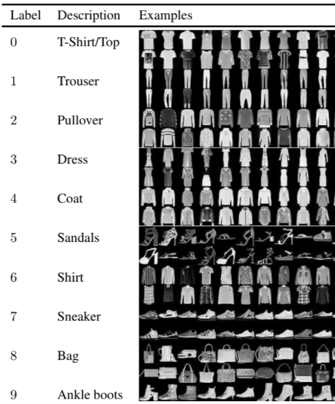
看线性改变三维坐标对生成图像影响
FashionMnist中所有的数据标签如下:
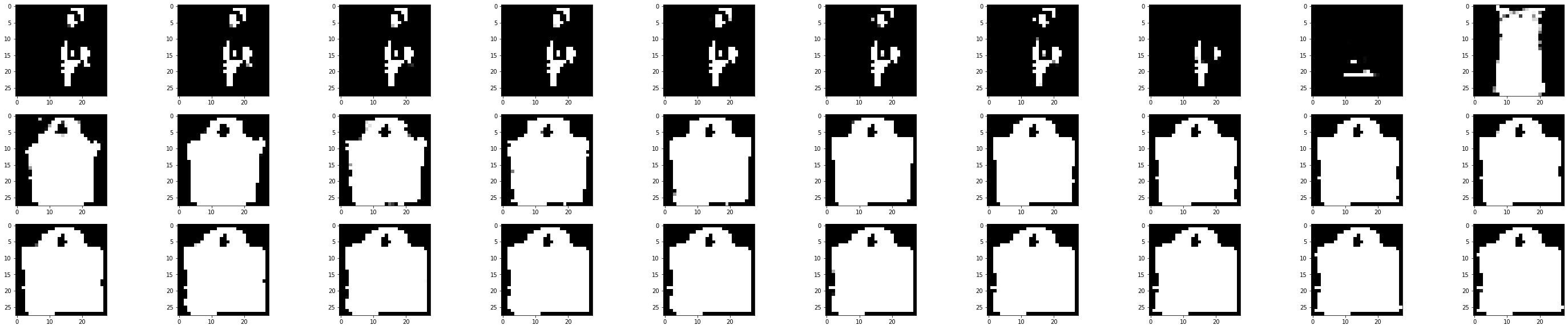
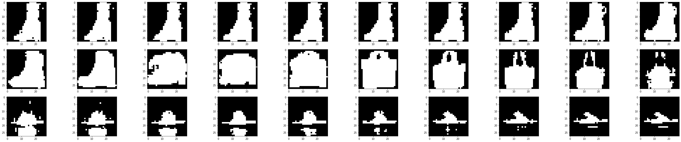
单独改变第一个维度
mask = np.array([1,0,0])
plt.figure(figsize=(50,10))
for i in range(30):
  tmp = rand_np + mask * (i - 15) * 500
  tensor = torch.from_numpy(tmp).float().to(device)
  # 得到encoded 测试集
  model.eval() # Set model to evaluation mode
  with torch.no_grad(): # Disable gradient calculation
      # Forward pass to get reconstructed output
      img = model.decoder(tensor)
      img_np = img.cpu().numpy()
  plt.subplot(3,10,i+1)
  plt.imshow(img_np.reshape(28,28), cmap='gray')
plt.show()
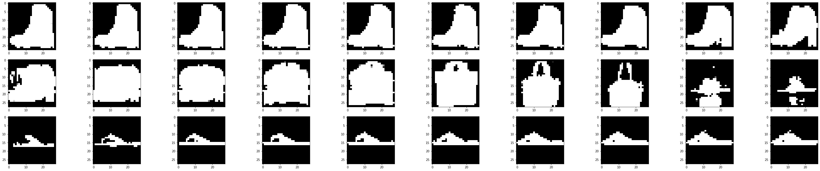
我们可以看到靴子-->高跟鞋-->手提袋-->包包-->帽子-->拖鞋,每两个相邻的图片之间可能只有细微的差别而已,但是我们的网络学会了把相似的东西放在了一起(而不是分散到两个地方)
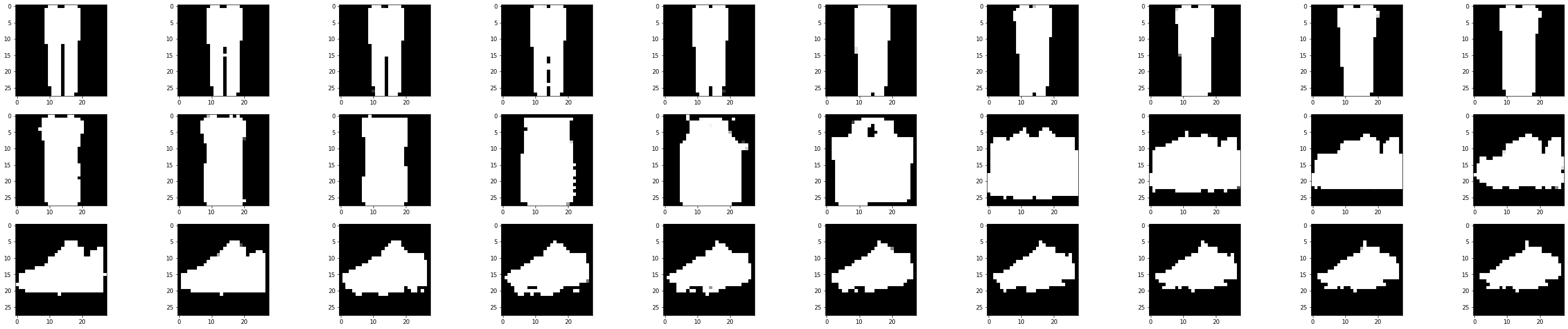
单独改变第二个维度
mask = np.array([0,1,0])
plt.figure(figsize=(50,10))
for i in range(30):
  tmp = rand_np + mask * (i - 15) * 500
  tensor = torch.from_numpy(tmp).float().to(device)
  # 得到encoded 测试集
  model.eval() # Set model to evaluation mode
  with torch.no_grad(): # Disable gradient calculation
      # Forward pass to get reconstructed output
      img = model.decoder(tensor)
      img_np = img.cpu().numpy()
  plt.subplot(3,10,i+1)
  plt.imshow(img_np.reshape(28,28), cmap='gray')
plt.show()
这个维度就没有太多的变化、类别之间变化也比较少,从一个奇怪的东西变成裙子再到包包所在的空间
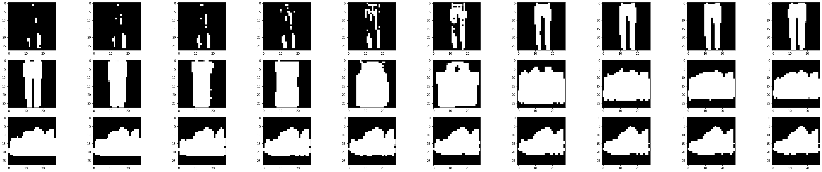
单独改变第三个维度
mask = np.array([0,0,1])
plt.figure(figsize=(50,10))
for i in range(30):
  tmp = rand_np + mask * (i - 15) * 500
  tensor = torch.from_numpy(tmp).float().to(device)
  # 得到encoded 测试集
  model.eval() # Set model to evaluation mode
  with torch.no_grad(): # Disable gradient calculation
      # Forward pass to get reconstructed output
      img = model.decoder(tensor)
      img_np = img.cpu().numpy()
  plt.subplot(3,10,i+1)
  plt.imshow(img_np.reshape(28,28), cmap='gray')
plt.show()
裤子-->裙子-->包包-->鞋子
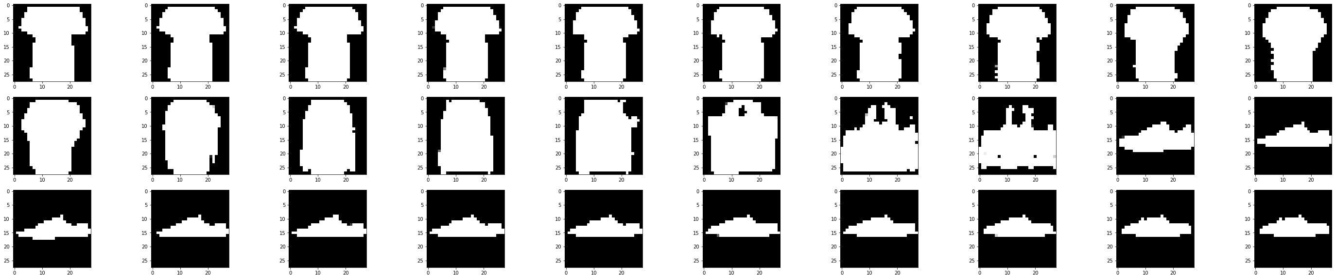
同时改变二、三维度
mask = np.array([0,1,1])
plt.figure(figsize=(50,10))
for i in range(30):
  tmp = rand_np + mask * (i - 15) * 500
  tensor = torch.from_numpy(tmp).float().to(device)
  # 得到encoded 测试集
  model.eval() # Set model to evaluation mode
  with torch.no_grad(): # Disable gradient calculation
      # Forward pass to get reconstructed output
      img = model.decoder(tensor)
      img_np = img.cpu().numpy()
  plt.subplot(3,10,i+1)
  plt.imshow(img_np.reshape(28,28), cmap='gray')
plt.show()
同时改变一、三维度
mask = np.array([1,0,1])
plt.figure(figsize=(50,10))
for i in range(30):
  tmp = rand_np + mask * (i - 15) * 500
  tensor = torch.from_numpy(tmp).float().to(device)
  # 得到encoded 测试集
  model.eval() # Set model to evaluation mode
  with torch.no_grad(): # Disable gradient calculation
      # Forward pass to get reconstructed output
      img = model.decoder(tensor)
      img_np = img.cpu().numpy()
  plt.subplot(3,10,i+1)
  plt.imshow(img_np.reshape(28,28), cmap='gray')
plt.show()
同时改变一、二维度
mask = np.array([1,1,0])
plt.figure(figsize=(50,10))
for i in range(30):
  tmp = rand_np + mask * (i - 15) * 500
  tensor = torch.from_numpy(tmp).float().to(device)
  # 得到encoded 测试集
  model.eval() # Set model to evaluation mode
  with torch.no_grad(): # Disable gradient calculation
      # Forward pass to get reconstructed output
      img = model.decoder(tensor)
      img_np = img.cpu().numpy()
  plt.subplot(3,10,i+1)
  plt.imshow(img_np.reshape(28,28), cmap='gray')
plt.show()
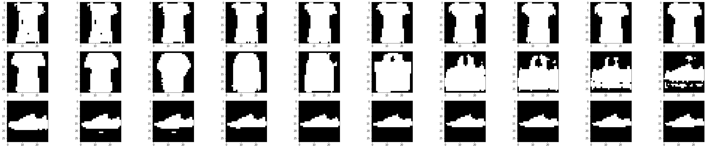
同时改变一、二、三维度
mask = np.array([1,1,1])
plt.figure(figsize=(50,10))
for i in range(30):
  tmp = rand_np + mask * (i - 15) * 500
  tensor = torch.from_numpy(tmp).float().to(device)
  # 得到encoded 测试集
  model.eval() # Set model to evaluation mode
  with torch.no_grad(): # Disable gradient calculation
      # Forward pass to get reconstructed output
      img = model.decoder(tensor)
      img_np = img.cpu().numpy()
  plt.subplot(3,10,i+1)
  plt.imshow(img_np.reshape(28,28), cmap='gray')
plt.show()

 浙公网安备 33010602011771号