吴恩达机器学习第一周讲义及自己理解
Machine Learning by Andrew Ng
- Machine Learning by Andrew Ng
- Supervised Learning
- Unsupervised Learning
- Frequently Asked Questions
- Model Representation
- Cost Function
- Cost Function - Intuition I
- Cost Function - Intuition II
- Gradient Descent
- Gradient Descent Intuition
- Gradient Descent For Linear Regression
- Matrices and Vectors
- Addition and Scalar Multiplication
- Matrix Vector Multiplication
- Matrix-Matrix Multiplication
- Matrix Multiplication Properties
- Inverse and Transpose
What is Machine Learning?
Two definitions of Machine Learning are offered. Arthur Samuel described it as: "the field of study that gives computers the ability to learn without being explicitly programmed." This is an older, informal definition.
Tom Mitchell provides a more modern definition: "A computer program is said to learn from experience E with respect to some class of tasks T and performance measure P, if its performance at tasks in T, as measured by P, improves with experience E."
Andrew Ng said that the sentence above maybe just make it rhyme.
Example: playing checkers.
E = the experience of playing many games of checkers
T = the task of playing checkers.
P = the probability that the program will win the next game.
In general, any machine learning problem can be assigned to one of two broad classifications:
Supervised learning and Unsupervised learning. (And some other methods like Reinforcement learning and Recommender systems)
Supervised Learning
Supervised Learning
In supervised learning, we are given a data set and already know what our correct output should look like, having the idea that there is a relationship between the input and the output.
Supervised learning problems are categorized into "regression" and "classification" problems. In a regression problem, we are trying to predict results within a continuous output, meaning that we are trying to map input variables to some continuous function. In a classification problem, we are instead trying to predict results in a discrete output. In other words, we are trying to map input variables into discrete categories.
Example 1:
Given data about the size of houses on the real estate market, try to predict their price. Price as a function of size is a continuous output, so this is a regression problem.
We could turn this example into a classification problem by instead making our output about whether the house "sells for more or less than the asking price." Here we are classifying the houses based on price into two discrete(离散的) categories.
Example 2:
(a) Regression - Given a picture of a person, we have to predict their age on the basis of the given picture
(b) Classification - Given a patient with a tumor, we have to predict whether the tumor is malignant(恶性的) or benign(良性的).
Unsupervised Learning
Unsupervised Learning
Unsupervised learning allows us to approach problems with little or no idea what our results should look like. We can derive structure from data where we don't necessarily know the effect of the variables.
We can derive this structure by clustering(聚类) the data based on relationships among the variables in the data.
With unsupervised learning there is no feedback based on the prediction results.
Example:
Clustering: Take a collection of 1,000,000 different genes, and find a way to automatically group these genes into groups that are somehow similar or related by different variables, such as lifespan, location, roles, and so on.
Non-clustering: The "Cocktail Party Algorithm", allows you to find structure in a chaotic environment. (i.e. identifying individual voices and music from a mesh of sounds at a cocktail party).
Frequently Asked Questions
The following Machine Learning Mentors(导师顾问) volunteered time to compile this list of Frequently Asked Questions: Colin Beckingham, Kevin Burnham, Maxim Haytovich, Tom Mosher, Richard Gayle, Simon Crase, Michael Reardon and Paul Mielke.
Be sure to thank them when you see them in the discussion forums!
General Questions
Q: Is the grader server down? A: First step is to check here.
Q: The audio in the videos is quite bad sometimes, muffled or low volume. Please fix it. A: You can mitigate(减轻) the audio issues by turning down the bass and up the treble if you have those controls, or using a headset, which naturally emphasizes the higher frequencies. Also you may want to switch on the English closed captioning. It is unlikely to be fixed in the near term because most students do not have serious problems and therefore it is low on the priority list.
*Q: What does it mean when I see “Math Processing Error?”* A: The page is attempting to use MathJax to render math symbols. Sometimes the content delivery network can be sluggish or you have caught the web page Ajax javascript code in an incomplete state. Normally just refreshing the page to make it load fully fixes the problem
*Q: How can I download lectures?* A: On Demand videos cannot be downloaded.
*Q: Is there a prerequisite(pre-requisition先决要求) for this course?*A: Students are expected to have the following background:
-
Knowledge of basic computer science principles and skills, at a level sufficient to write a reasonably non-trivial computer program.
-
Familiarity with the basic probability theory.
-
Familiarity with the basic linear algebra.
*Q: Why do we have to use Matlab or Octave? Why not Clojure, Julia, Python, R or [Insert favourite language here]?*A: As Prof. Ng explained in the 1st video of the Octave tutorial, he has tried teaching Machine Learning in a variety of languages, and found that students come up to speed faster with Matlab/Octave. Therefore the course was designed using Octave/Matlab, and the automatic submission grader uses those program interfaces. Octave and Matlab are optimized for rapid vectorized calculations, which is very useful in Machine Learning. R is a nice tool, but:
- It is a bit too high level. This course shows how to actually implement the algorithms of machine learning, while R already has them implemented. Since the focus of this course is to show you what happens in ML algorithms under the hood, you need to use Octave 2. This course offers some starter code in Octave/Matlab, which will really save you tons of time solving the tasks.
*Q: Has anyone figured out the how to solve this problem? Here is my code [Insert code].* A: This is a violation of the Coursera Honor Code. Find the Honor Code here.
*Q: I've submitted correct answers for [insert problem]. However I would like to compare my implementation with other who did correctly.* A: This is a violation of the Coursera Honor Code. Find the Honor Code here.
*Q: This is my email: [insert email]. Can we get the answer for the quiz?* A: This is a violation of the Coursera Honor Code. Find the Honor Code here.
Q: Do I receive a certificate once I complete this course? A: Course Certificate is available in this course. Click here to learn about how Course Certificate works and how to purchase.
*Q: Why do all the answers in a multiple correct question say correct response when you submit the answer to an in-video question?* A: Coursera's software is designed to suggest the correctness of each state of the check box. Therefore, an answer having a correct answer tag below it means that the state of that check box is correct.
*Q: What is the correct technique of entering a numeric answer to a text box question ?* A: Coursera's software for numeric answers only supports '.' as the decimal delimiter (not ',') and require that fractions be simplified to decimals. For answers with many decimal digits, please use a 2 digits after decimal point rounding method when entering solutions if not mentioned in the question.
*Q: What is the correct technique of entering a 1 element matrix ?* A: They should be entered as just the element without brackets.
*Q: What does a A being a 3 element vector or a 3 dimensional vector mean?* A: If not described a vector as mentioned in the questions is \(A=[element1\;element2\;element3]\)
*Q: I think I found an error in a video. What should I do?* A: First, check the errata section under resources menu. If you are unsure if it is an error, create a new thread in the discussion forum describing the error.
*Q: My quiz grade displayed is wrong or I have a verification issue or I cannot retake a quiz. What should I do?* A: Contact Help Center. These queries can only be resolved by learner support and it is best if they are contacted directly.
Model Representation
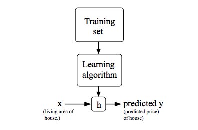
To establish notation for future use, we’ll use \(x^{(i)}\) to denote the “input” variables (living area in this example), also called input features, and \(y^{(i)}\)to denote the “output” or target variable that we are trying to predict (price). A pair \((x^{(i)} , y^{(i)} )\) is called a training example, and the dataset that we’ll be using to learn—a list of m training examples \((x^{(i)} , y^{(i)}); i = 1, . . . , m\)}—is called a training set. Note that the superscript “(i)” in the notation is simply an index into the training set, and has nothing to do with exponentiation. We will also use X to denote the space of input values, and Y to denote the space of output values. In this example, X = Y = ℝ.
To describe the supervised learning problem slightly more formally, our goal is, given a training set, to learn a function h : X → Y so that h(x) is a “good” predictor for the corresponding value of y. For historical reasons, this function h is called a hypothesis. Seen pictorially, the process is therefore like this:
When the target variable that we’re trying to predict is continuous, such as in our housing example, we call the learning problem a regression problem. When y can take on only a small number of discrete values (such as if, given the living area, we wanted to predict if a dwelling is a house or an apartment, say), we call it a classification problem.
Cost Function
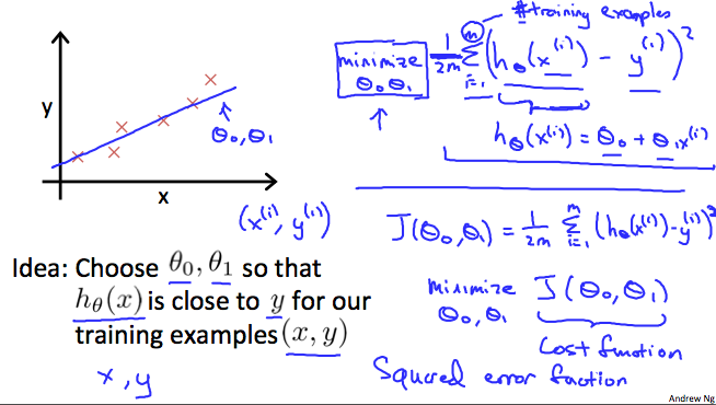
We can measure the accuracy of our hypothesis function by using a cost function. This takes an average difference (actually a fancier version of an average) of all the results of the hypothesis with inputs from x's and the actual output y's.
To break it apart, it is \(\frac{1}{2}\) \(\bar{x}\) where \(\bar{x}\) is the mean of the squares of \(h_\theta (x_{i}) - y_{i}\) , or the difference between the predicted value and the actual value.
This function is otherwise called the "Squared error function", or "Mean squared error". The mean is halved \(\left( \frac{1}{2}\right)\) as a convenience for the computation of the gradient descent, as the derivative term of the square function will cancel out the \(\frac{1}{2}\) term. The following image summarizes what the cost function does:
Connecting to what we have learned in the high school we found that \(h_{\theta}(x)\rightarrow \hat{y}\) and \(h_{\theta}(x_i)\rightarrow \hat{y_i}\)
Cost Function - Intuition I
If we try to think of it in visual terms, our training data set is scattered on the x-y plane. We are trying to make a straight line (defined by \(h_\theta(x)\) )which passes through these scattered data points.
Our objective is to get the best possible line. The best possible line will be such so that the average squared vertical distances of the scattered points from the line will be the least. Ideally, the line should pass through all the points of our training data set. In such a case, the value of \(J(\theta_0, \theta_1)\) will be 0. The following example shows the ideal situation where we have a cost function of 0.
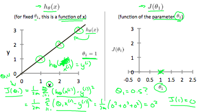
When \(\theta_1 = 1\), we get a slope of 1 which goes through every single data point in our model. Conversely, when \(\theta_1 = 0.5\), we see the vertical distance from our fit to the data points increase.
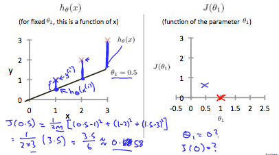
This increases our cost function to 0.58. Plotting several other points yields to the following graph:
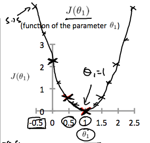
Thus as a goal, we should try to minimize the cost function. In this case, \(\theta_1 = 1\) is our global minimum.
Cost Function - Intuition II
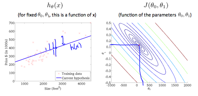
A contour plot is a graph that contains many contour lines. A contour line of a two variable function has a constant value at all points of the same line. An example of such a graph is the one to the right below.
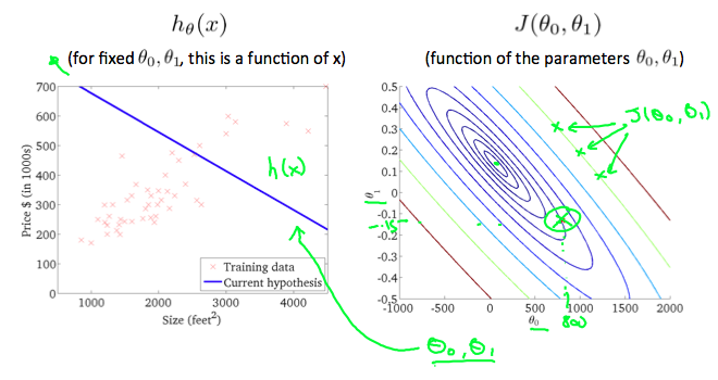
Taking any color and going along the 'circle', one would expect to get the same value of the cost function. For example, the three green points found on the green line above have the same value for \(J(\theta_0,\theta_1)\) and as a result, they are found along the same line. The circled x displays the value of the cost function for the graph on the left when \(\theta_0 = 800\) and \(\theta_1= -0.15\). Taking another \(h(x)\) and plotting its contour plot, one gets the following graphs:
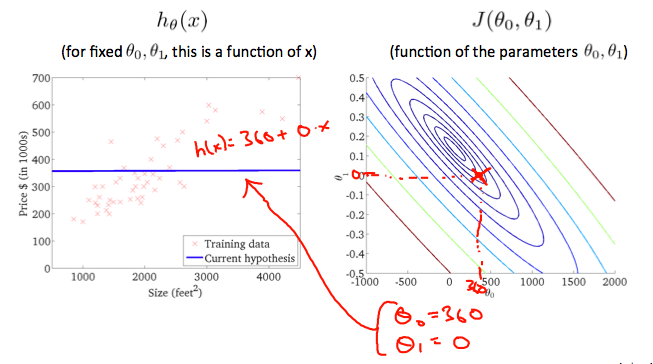
When \(\theta_0 = 360\) and \(\theta_1 = 0\), the value of \(J(\theta_0,\theta_1)\) in the contour plot gets closer to the center thus reducing the cost function error. Now giving our hypothesis function a slightly positive slope results in a better fit of the data.
The graph above minimizes the cost function as much as possible and consequently, the result of \(\theta_1\)and \(\theta_0\) tend to be around 0.12 and 250 respectively. Plotting those values on our graph to the right seems to put our point in the center of the inner most 'circle'.
Gradient Descent
So we have our hypothesis function and we have a way of measuring how well it fits into the data. Now we need to estimate the parameters in the hypothesis function. That's where gradient descent comes in.
Imagine that we graph our hypothesis function based on its fields \(\theta_0\) and \(\theta_1\) (actually we are graphing the cost function as a function of the parameter estimates). We are not graphing x and y itself, but the parameter range of our hypothesis function and the cost resulting from selecting a particular set of parameters.
We put \(\theta_0\) on the x axis and \(\theta_1\) on the y axis, with the cost function on the vertical z axis. The points on our graph will be the result of the cost function using our hypothesis with those specific theta parameters. The graph below depicts(描绘) such a setup.
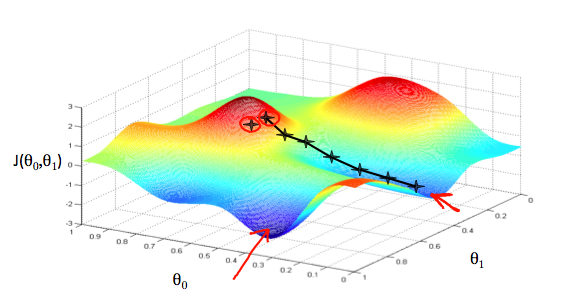
We will know that we have succeeded when our cost function is at the very bottom of the pits in our graph, i.e. when its value is the minimum. The red arrows show the minimum points in the graph.
The way we do this is by taking the derivative (the tangential line to a function) of our cost function. The slope of the tangent is the derivative at that point and it will give us a direction to move towards. We make steps down the cost function in the direction with the steepest descent. The size of each step is determined by the parameter α, which is called the learning rate.
For example, the distance between each 'star' in the graph above represents a step determined by our parameter α. A smaller α would result in a smaller step and a larger α results in a larger step. The direction in which the step is taken is determined by the partial derivative of \(J(\theta_0,\theta_1)\). Depending on where one starts on the graph, one could end up at different points. The image above shows us two different starting points that end up in two different places.
The gradient descent algorithm is:
repeat until convergence(收敛):
\(\theta_j := \theta_j - \alpha \frac{\partial}{\partial \theta_j} J(\theta_0, \theta_1)\)
where
j=0,1 represents the feature index number.
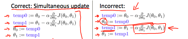
At each iteration j, one should simultaneously update the parameters \(\theta_1, \theta_2,...,\theta_n\). Updating a specific parameter prior to calculating another one on the $j^{(th)} $iteration(迭代) would yield to a wrong implementation.
Gradient Descent Intuition
In this video we explored the scenario(预想) where we used one parameter \(\theta_1\) and plotted its cost function to implement a gradient descent. Our formula for a single parameter was :
Repeat until convergence:
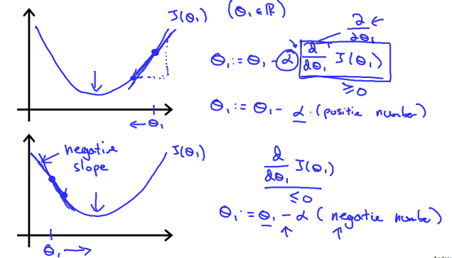
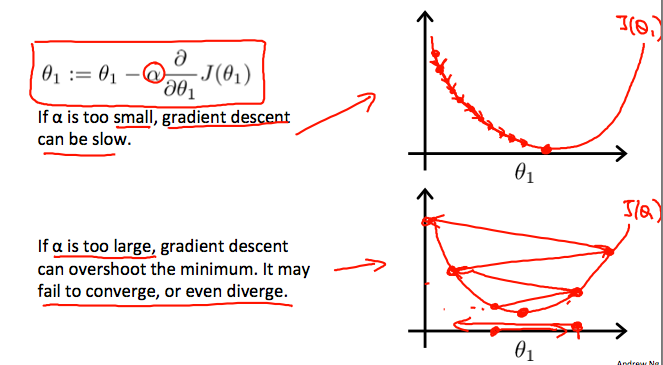
$\theta_1:=\theta_1-\alpha \frac{d}{d\theta_1}J(\theta_1) $
Regardless of the slope's sign for \(\frac{d}{d\theta_1}\), \(\theta_1\) eventually converges to its minimum value. The following graph shows that when the slope is negative, the value of \(\theta_1\) increases and when it is positive, the value of \(\theta_1\) decreases.
On a side note, we should adjust our parameter \(\alpha\) to ensure that the gradient descent algorithm converges in a reasonable time. Failure to converge or too much time to obtain the minimum value imply that our step size is wrong.
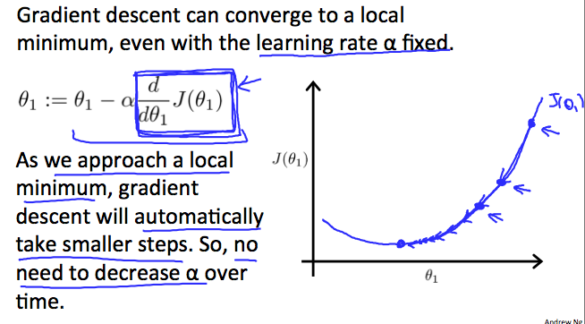
How does gradient descent converge with a fixed step size \(\alpha\)?
The intuition behind the convergence is that \(\frac{d}{d\theta_1} J(\theta_1)\) approaches 0 as we approach the bottom of our convex function. At the minimum, the derivative will always be 0 and thus we get:
\(\theta_1:=\theta_1-\alpha * 0\)
In the gif here, you can see the Gradient Descent will get the best performance while $\alpha $ maybe equal to 0.26( it only need one iteration and get what it want ),
- if $\alpha $ is smaller, it takes more iterations but could not get the same performance(it's hard to get minimum).
- if $\alpha $ is a bit larger, in some cases, it also can get the same speed as the smaller-alpha one, however, when it larger than some values, it will never converge to the local minimum.
- In my opinion, to limit the area of $ \alpha $ at the beginning is very necessary.
Gradient Descent For Linear Regression
Note: [At 6:15 "h(x) = -900 - 0.1x" should be "h(x) = 900 - 0.1x"]
When specifically applied to the case of linear regression, a new form of the gradient descent equation can be derived. We can substitute our actual cost function and our actual hypothesis function and modify the equation to :
where m is the size of the training set, $ \theta_0$ a constant that will be changing simultaneously with $ \theta_1$ and \(x_{i}, y_{i}\)are values of the given training set (data).
Note that we have separated out the two cases for \(\theta_j\) into separate equations for $ \theta_0$ and $ \theta_1$; and that for $ \theta_1 $ we are multiplying \(x_{i}\) at the end due to the derivative. The following is a derivation of $\frac {\partial}{\partial \theta_j} $for a single example :
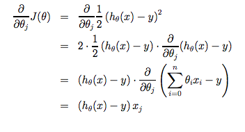
The point of all this is that if we start with a guess for our hypothesis and then repeatedly apply these gradient descent equations, our hypothesis will become more and more accurate.
So, this is simply gradient descent on the original cost function J. This method looks at every example in the entire training set on every step, and is called batch(批量) gradient descent. Note that, while gradient descent can be susceptible to local minima in general, the optimization problem we have posed here for linear regression has only one global, and no other local, optima; thus gradient descent always converges (assuming the learning rate α is not too large) to the global minimum. Indeed, J is a convex quadratic(平方的) function. Here is an example of gradient descent as it is run to minimize a quadratic function.
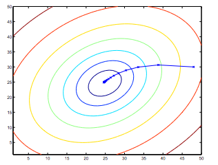
The ellipses shown above are the contours of a quadratic function. Also shown is the trajectory taken by gradient descent, which was initialized at (48,30). The x’s in the figure (joined by straight lines) mark the successive values of θ that gradient descent went through as it converged to its minimum.
Matrices and Vectors
Matrices are 2-dimensional arrays:
The above matrix has four rows and three columns, so it is a 4 x 3 matrix.
A vector is a matrix with one column and many rows:
So vectors are a subset of matrices. The above vector is a 4 x 1 matrix.
Notation and terms:
- \(A_{ij}\) refers to the element in the ith row and jth column of matrix A.
- A vector with 'n' rows is referred to as an 'n'-dimensional vector.
- \(v_i\) refers to the element in the ith row of the vector.
- In general, all our vectors and matrices will be 1-indexed. Note that for some programming languages, the arrays are 0-indexed.
- Matrices are usually denoted by uppercase names while vectors are lowercase.
- "Scalar" means that an object is a single value, not a vector or matrix.
- \(\mathbb{R}\) refers to the set of scalar(标量) real numbers.
- \(\mathbb{R^n}\) refers to the set of n-dimensional vectors of real numbers.
Run the cell below to get familiar with the commands in Octave/Matlab. Feel free to create matrices and vectors and try out different things.
% The ; denotes we are going back to a new row.
A = [1, 2, 3; 4, 5, 6; 7, 8, 9; 10, 11, 12]

% Initialize a vector
v = [1;2;3]

% Get the dimension of the matrix A where m = rows and n = columns
[m,n] = size(A)

% You could also store it this way
dim_A = size(A)

% Get the dimension of the vector v
dim_v = size(v)

% Now let's index into the 2nd row 3rd column of matrix A
A_23 = A(2,3)
Addition and Scalar Multiplication
Addition and subtraction are element-wise, so you simply add or subtract each corresponding element:
Subtracting Matrices:
To add or subtract two matrices, their dimensions must be the same.
In scalar multiplication, we simply multiply every element by the scalar value:
In scalar division, we simply divide every element by the scalar value:
Experiment below with the Octave/Matlab commands for matrix addition and scalar multiplication. Feel free to try out different commands. Try to write out your answers for each command before running the cell below.
% Initialize matrix A and B
A = [1, 2, 4; 5, 3, 2]
B = [1, 3, 4; 1, 1, 1]

% Initialize constant s
s = 2

% See how element-wise addition works
add_AB = A + B

% See how element-wise subtraction works
sub_AB = A - B

% See how scalar multiplication works
mult_As = A * s

% Divide A by s
div_As = A / s

% What happens if we have a Matrix + scalar?
add_As = A + s
Matrix Vector Multiplication
We map the column of the vector onto each row of the matrix, multiplying each element and summing the result.
The result is a vector. The number of columns of the matrix must equal the number of rows of the vector.
An \(m \times n\) matrix multiplied by an \(n \times 1\) vector results in an \(m \times 1\) vector.
Below is an example of a matrix-vector multiplication. Make sure you understand how the multiplication works. Feel free to try different matrix-vector multiplications.
% Initialize matrix A
A = [1, 2, 3; 4, 5, 6;7, 8, 9]

% Initialize vector v
v = [1; 1; 1]

% Multiply A * v
Av = A * v
Matrix-Matrix Multiplication
We multiply two matrices by breaking it into several vector multiplications and concatenating the result.
An m x n matrix multiplied by an n x o matrix results in an m x o matrix. In the above example, a 3 x 2 matrix times a 2 x 2 matrix resulted in a 3 x 2 matrix.
To multiply two matrices, the number of columns of the first matrix must equal the number of rows of the second matrix.
For example:
% Initialize a 3 by 2 matrix
A = [1, 2; 3, 4;5, 6]

% Initialize a 2 by 1 matrix
B = [1; 2]

% We expect a resulting matrix of (3 by 2)*(2 by 1) = (3 by 1)
mult_AB = A*B

% Make sure you understand why we got that result
Matrix Multiplication Properties
- Matrices are not commutative: \(A∗B \neq B∗A\)
- Matrices are associative(结合的): \((A∗B)∗C = A∗(B∗C)\)
The identity matrix, when multiplied by any matrix of the same dimensions, results in the original matrix. It's just like multiplying numbers by 1. The identity matrix simply has 1's on the diagonal (upper left to lower right diagonal) and 0's elsewhere.
\(\begin{bmatrix}1&0&0\\0&1&0\\0&0&1\\\end{bmatrix}\)
When multiplying the identity matrix after some matrix (A∗I), the square identity matrix's dimension should match the other matrix's columns. When multiplying the identity matrix before some other matrix (I∗A), the square identity matrix's dimension should match the other matrix's rows.
% Initialize random matrices A and B
A = [1,2;4,5]
B = [1,1;0,2]

% Initialize a 2 by 2 identity matrix
I = eye(2)

% The above notation is the same as I = [1,0;0,1]

% What happens when we multiply I*A ?
IA = I*A

% How about A*I ?
AI = A*I

% Compute A*B
AB = A*B

% Is it equal to B*A?
BA = B*A

% Note that IA = AI but AB != BA
Inverse and Transpose
The inverse of a matrix A is denoted \(A^{-1}\). Multiplying by the inverse results in the identity matrix.
A non square matrix does not have an inverse matrix. We can compute inverses of matrices in octave with the \(pinv(A)\) function and in Matlab with the \(inv(A)\) function. Matrices that don't have an inverse are singular or degenerate.
The transposition of a matrix is like rotating the matrix 90° in clockwise direction and then reversing it. We can compute transposition of matrices in matlab with the transpose(A) function or A':
In other words:
\(A_{ij} = A^T_{ji}\)
% Initialize matrix A
A = [1,2,0;0,5,6;7,0,9]

% Transpose A
A_trans = A'

% Take the inverse of A
A_inv = inv(A)

% What is A^(-1)*A?
A_invA = inv(A)*A

 浙公网安备 33010602011771号