Pytorch深入学习阶段二（二）

Pytorch学习阶段二（二）

学习Pytorch重要组成部分。

一、warm-up：numpy#

下式将被用于本篇计算当中：

y = a + b x^{2} + c x^{3}

$y = a+bx^2+cx^3$

手算BP和gradient descen：

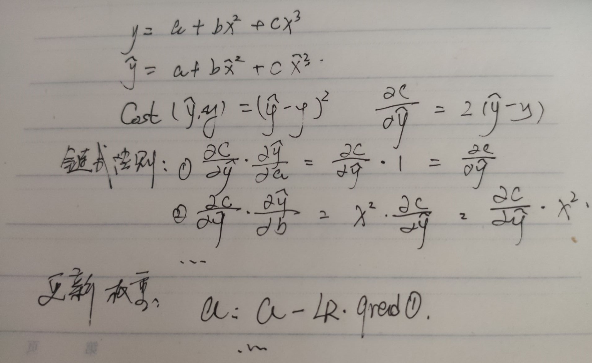
运用numpy模拟神经网络训练的过程，这个过程中，可以解为线性拟合的过程。

# -*- coding: utf-8 -*-
import numpy as np
import math

# Create random input and output data
x = np.linspace(-math.pi, math.pi, 2000)
y = np.sin(x)

# Randomly initialize weights
a = np.random.randn()
b = np.random.randn()
c = np.random.randn()
d = np.random.randn()

learning_rate = 1e-6
for t in range(2000):
    # Forward pass: compute predicted y
    # y = a + b x + c x^2 + d x^3
    y_pred = a + b * x + c * x ** 2 + d * x ** 3

    # Compute and print loss
    loss = np.square(y_pred - y).sum()
    if t % 100 == 99:
        print(t, loss)

    # Backprop to compute gradients of a, b, c, d with respect to loss
    # 此处用到了链式法则来计算的，如上图
    grad_y_pred = 2.0 * (y_pred - y)
    grad_a = grad_y_pred.sum()
    grad_b = (grad_y_pred * x).sum()
    grad_c = (grad_y_pred * x ** 2).sum()
    grad_d = (grad_y_pred * x ** 3).sum()

    # Update weights
    a -= learning_rate * grad_a
    b -= learning_rate * grad_b
    c -= learning_rate * grad_c
    d -= learning_rate * grad_d

print(f'Result: y = {a} + {b} x + {c} x^2 + {d} x^3')

>>>
Result: y = 0.023675257391932762 + 0.8118703877064724 x + -0.004084375858091895 x^2 + -0.08694795749996177 x^3

通过gradient descent来更新权重。

二、Tensor#

虽然numpy不能在GPU上训练，但是其升级版Tensor，可以用GPU加速。

# -*- coding: utf-8 -*-

import torch
import math


dtype = torch.float
device = torch.device("cpu")
# device = torch.device("cuda:0") # Uncomment this to run on GPU

# Create random input and output data
x = torch.linspace(-math.pi, math.pi, 2000, device=device, dtype=dtype)
y = torch.sin(x)

# Randomly initialize weights
a = torch.randn((), device=device, dtype=dtype)
b = torch.randn((), device=device, dtype=dtype)
c = torch.randn((), device=device, dtype=dtype)
d = torch.randn((), device=device, dtype=dtype)

learning_rate = 1e-6
for t in range(2000):
    # Forward pass: compute predicted y
    y_pred = a + b * x + c * x ** 2 + d * x ** 3

    # Compute and print loss
    loss = (y_pred - y).pow(2).sum().item()
    if t % 100 == 99:
        print(t, loss)

    # Backprop to compute gradients of a, b, c, d with respect to loss
    grad_y_pred = 2.0 * (y_pred - y)
    grad_a = grad_y_pred.sum()
    grad_b = (grad_y_pred * x).sum()
    grad_c = (grad_y_pred * x ** 2).sum()
    grad_d = (grad_y_pred * x ** 3).sum()

    # Update weights using gradient descent
    a -= learning_rate * grad_a
    b -= learning_rate * grad_b
    c -= learning_rate * grad_c
    d -= learning_rate * grad_d


print(f'Result: y = {a.item()} + {b.item()} x + {c.item()} x^2 + {d.item()} x^3')

三、Autograd#

上述两种方式，用手算的方法计算了函数的链式法则和梯度更新。那利用autograd计算梯度是怎样的？autograd运用到计算图，而计算图用来记录一了函数的计算步骤，BP通过这张图就可以反向算出其梯度。

# -*- coding: utf-8 -*-
import torch
import math

dtype = torch.float
device = torch.device("cpu")
# device = torch.device("cuda:0")  # Uncomment this to run on GPU

# Create Tensors to hold input and outputs.
# By default, requires_grad=False, which indicates that we do not need to
# compute gradients with respect to these Tensors during the backward pass.
x = torch.linspace(-math.pi, math.pi, 2000, device=device, dtype=dtype)
y = torch.sin(x)

# Create random Tensors for weights. For a third order polynomial, we need
# 4 weights: y = a + b x + c x^2 + d x^3
# Setting requires_grad=True indicates that we want to compute gradients with
# respect to these Tensors during the backward pass.
a = torch.randn((), device=device, dtype=dtype, requires_grad=True)
b = torch.randn((), device=device, dtype=dtype, requires_grad=True)
c = torch.randn((), device=device, dtype=dtype, requires_grad=True)
d = torch.randn((), device=device, dtype=dtype, requires_grad=True)

learning_rate = 1e-6
for t in range(2000):
    # Forward pass: compute predicted y using operations on Tensors.
    y_pred = a + b * x + c * x ** 2 + d * x ** 3

    # Compute and print loss using operations on Tensors.
    # Now loss is a Tensor of shape (1,)
    # loss.item() gets the scalar value held in the loss.
    loss = (y_pred - y).pow(2).sum()
    if t % 100 == 99:
        print(t, loss.item())

    # Use autograd to compute the backward pass. This call will compute the
    # gradient of loss with respect to all Tensors with requires_grad=True.
    # After this call a.grad, b.grad. c.grad and d.grad will be Tensors holding
    # the gradient of the loss with respect to a, b, c, d respectively.
    loss.backward()

    # Manually update weights using gradient descent. Wrap in torch.no_grad()
    # because weights have requires_grad=True, but we don't need to track this
    # in autograd.
    with torch.no_grad():
        a -= learning_rate * a.grad
        b -= learning_rate * b.grad
        c -= learning_rate * c.grad
        d -= learning_rate * d.grad

        # Manually zero the gradients after updating weights
        a.grad = None
        b.grad = None
        c.grad = None
        d.grad = None

print(f'Result: y = {a.item()} + {b.item()} x + {c.item()} x^2 + {d.item()} x^3')

四、定义autograd functions#

每个原始的autograd都是由两个函数操作张量，一个向前传播计算输入，一个后向传播计算梯度，以此更新权值。在pytorch中，我们可以简单的定义我们自己的autograd操作，通过定义torch.autograd.Function的子类，并重写forward和backward函数。

例如

P_{3} (x) = \frac{1}{2} (5 x^{3} - 3 x)

$P_3(x)= \frac{1}{2}(5x^3−3x)$

复杂求导，可以重写函数，具体如下。

# -*- coding: utf-8 -*-
import torch
import math


class LegendrePolynomial3(torch.autograd.Function):
    """
    We can implement our own custom autograd Functions by subclassing
    torch.autograd.Function and implementing the forward and backward passes
    which operate on Tensors.
    """

    @staticmethod
    def forward(ctx, input):
        """
        In the forward pass we receive a Tensor containing the input and return
        a Tensor containing the output. ctx is a context object that can be used
        to stash information for backward computation. You can cache arbitrary
        objects for use in the backward pass using the ctx.save_for_backward method.
        """
        ctx.save_for_backward(input)
        return 0.5 * (5 * input ** 3 - 3 * input)

    @staticmethod
    def backward(ctx, grad_output):
        """
        In the backward pass we receive a Tensor containing the gradient of the loss
        with respect to the output, and we need to compute the gradient of the loss
        with respect to the input.
        """
        input, = ctx.saved_tensors
        return grad_output * 1.5 * (5 * input ** 2 - 1)
...
...
learning_rate = 5e-6
for t in range(2000):
    # To apply our Function, we use Function.apply method. We alias this as 'P3'.
    P3 = LegendrePolynomial3.apply

    # Forward pass: compute predicted y using operations; we compute
    # P3 using our custom autograd operation.
    y_pred = a + b * P3(c + d * x)
...
...

五、nn.module#

计算图和autograd是一个非常强大的求导工具，但是大型深度网络，原始的autograd就有一点效率太低了。

在pytorch当中，nn包定义了一些模型，这可以大致地等同于神经网络层。nn同时也定义了一系列的有用的损失函数，这可以被用于训练圣经网络。

有人说3层的神经网络可以拟合出任何函数，下例表示拟合过程：

# -*- coding: utf-8 -*-
import torch
import math


# Create Tensors to hold input and outputs.
x = torch.linspace(-math.pi, math.pi, 2000)
y = torch.sin(x)

# For this example, the output y is a linear function of (x, x^2, x^3), so
# we can consider it as a linear layer neural network. Let's prepare the
# tensor (x, x^2, x^3).
p = torch.tensor([1, 2, 3])
xx = x.unsqueeze(-1).pow(p)

# In the above code, x.unsqueeze(-1) has shape (2000, 1), and p has shape
# (3,), for this case, broadcasting semantics will apply to obtain a tensor
# of shape (2000, 3) 

# Use the nn package to define our model as a sequence of layers. nn.Sequential
# is a Module which contains other Modules, and applies them in sequence to
# produce its output. The Linear Module computes output from input using a
# linear function, and holds internal Tensors for its weight and bias.
# The Flatten layer flatens the output of the linear layer to a 1D tensor,
# to match the shape of `y`.
model = torch.nn.Sequential(
    torch.nn.Linear(3, 1),
    torch.nn.Flatten(0, 1)
)

# The nn package also contains definitions of popular loss functions; in this
# case we will use Mean Squared Error (MSE) as our loss function.
loss_fn = torch.nn.MSELoss(reduction='sum')

learning_rate = 1e-6
for t in range(2000):

    # Forward pass: compute predicted y by passing x to the model. Module objects
    # override the __call__ operator so you can call them like functions. When
    # doing so you pass a Tensor of input data to the Module and it produces
    # a Tensor of output data.
    y_pred = model(xx)

    # Compute and print loss. We pass Tensors containing the predicted and true
    # values of y, and the loss function returns a Tensor containing the
    # loss.
    loss = loss_fn(y_pred, y)
    if t % 100 == 99:
        print(t, loss.item())

    # Zero the gradients before running the backward pass.
    model.zero_grad()

    # Backward pass: compute gradient of the loss with respect to all the learnable
    # parameters of the model. Internally, the parameters of each Module are stored
    # in Tensors with requires_grad=True, so this call will compute gradients for
    # all learnable parameters in the model.
    loss.backward()

    # Update the weights using gradient descent. Each parameter is a Tensor, so
    # we can access its gradients like we did before.
    with torch.no_grad():
        for param in model.parameters():
            param -= learning_rate * param.grad

# You can access the first layer of `model` like accessing the first item of a list
linear_layer = model[0]

# For linear layer, its parameters are stored as `weight` and `bias`.
print(f'Result: y = {linear_layer.bias.item()} + {linear_layer.weight[:, 0].item()} x + {linear_layer.weight[:, 1].item()} x^2 + {linear_layer.weight[:, 2].item()} x^3')

>>>
Result: y = -0.0036663166247308254 + 0.8344725966453552 x + 0.0006325002759695053 x^2 + -0.09016292542219162 x^3

六、优化器#

优化器简化了自己写更新权重的过程：

optimizer = torch.optim.RMSprop(model.parameters(), lr=learning_rate)
for t in range(2000):
    # Forward pass: compute predicted y by passing x to the model.
    y_pred = model(xx)

    # Compute and print loss.
    loss = loss_fn(y_pred, y)
    if t % 100 == 99:
        print(t, loss.item())

    # Before the backward pass, use the optimizer object to zero all of the
    # gradients for the variables it will update (which are the learnable
    # weights of the model). This is because by default, gradients are
    # accumulated in buffers( i.e, not overwritten) whenever .backward()
    # is called. Checkout docs of torch.autograd.backward for more details.
    optimizer.zero_grad()

    # Backward pass: compute gradient of the loss with respect to model
    # parameters
    loss.backward()

    # Calling the step function on an Optimizer makes an update to its
    # parameters
    optimizer.step()