Pytorch深入学习阶段二（一）

Pytorch学习二阶段

一、自动求导#

训练神经网络包含两步：

• 前向传播
• 后向传播：后向传播中，NN将调整他的参数，并通过loss_function来自计算误差，并通过优化器来优化参数。

import torch, torchvision
model = torchvision.models.resnet18(pretrained=True)
data = torch.rand(1, 3, 64, 64)
labels = torch.rand(1, 1000)

prediction = model(data) # forward pass

>>>data
tensor([[[[0.0792, 0.3683, 0.3258,  ..., 0.8572, 0.9326, 0.5032],
          [0.3238, 0.3992, 0.6769,  ..., 0.7879, 0.6261, 0.4239],
          [0.0839, 0.7466, 0.7469,  ..., 0.0616, 0.5267, 0.0221],
          ...,
          [0.4114, 0.2793, 0.4946,  ..., 0.3337, 0.0151, 0.9790],
          [0.4874, 0.2718, 0.3890,  ..., 0.6204, 0.2941, 0.9589],
          [0.8202, 0.3904, 0.9375,  ..., 0.1282, 0.2416, 0.0420]],

         [[0.2958, 0.6416, 0.2069,  ..., 0.0054, 0.3710, 0.8716],
          [0.2861, 0.6640, 0.3595,  ..., 0.4552, 0.6691, 0.9000],
          [0.1908, 0.1988, 0.0502,  ..., 0.9516, 0.0986, 0.2951],
          ...,
          [0.3542, 0.6152, 0.8829,  ..., 0.7102, 0.7418, 0.2471],
          [0.1259, 0.4121, 0.4195,  ..., 0.0277, 0.7919, 0.1961],
          [0.6761, 0.1635, 0.6317,  ..., 0.5082, 0.8117, 0.4959]],...
>>>labels
tensor([[9.7649e-01, 7.4230e-01, 8.9876e-01, 3.9301e-01, 4.3104e-01, 2.5916e-01,
         2.1638e-01, 2.3715e-01, 3.6239e-01, 5.1230e-02, 5.0033e-01, 9.3420e-01,
         7.3738e-01, 5.1232e-01, 6.1602e-01, 3.1946e-01, 3.3043e-01, 6.6394e-01,
         6.5134e-01, 4.4163e-01, 3.2559e-01, 1.1167e-01, 9.5033e-01, 2.6302e-01,
         4.9590e-01, 1.1047e-01, 6.7810e-01, 1.6822e-01, 3.9666e-01, 9.3511e-01,...
   

计算完毕前向传播后，通过与真实标签计算误差（目前常用交叉熵去计算）。然后下一步就是后向传播误差在网络参数中，自动梯度计算并存储了梯度为每个参数，通过.grad属性。

loss = (prediction - labels).sum()
loss.backward() # backward pass

>>> loss
tensor(-491.3782, grad_fn=<SumBackward0>)

接下来定义优化器，用随机梯度下降，SGD，并且Learning_rate设置为0.01，动量设置为0.9。

optim = torch.optim.SGD(model.parameters(), lr=1e-2, momentum=0.9)

>>> optim
SGD (
Parameter Group 0
    dampening: 0
    lr: 0.01
    momentum: 0.9
    nesterov: False
    weight_decay: 0
)

最后我们调用.step()来初始玩成梯度下降，优化器最后会调整参数通过模型属性.grad。

optim.step() #gradient descent

（一）Autograd中的微分#

autograd是怎样收集梯度的呢？

举例如下：

import torch

a = torch.tensor([2., 3.], requires_grad=True)
b = torch.tensor([6., 4.], requires_grad=True)

$$Q=3a^3-b^2$$

假设a，b都是NN的参数，Q是损失，在训练过程，优化参数求导：

$$\frac{∂Q}{∂a}=9a^2$$

$$\frac{∂Q}{∂b}=-2b$$

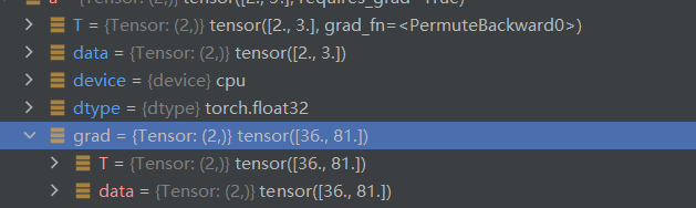
当调用.backward()在Q上，autograd计算这些梯度和分数，在参数的.grad属性。

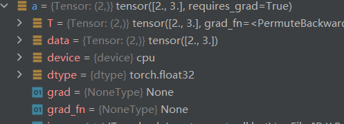
在idea中可以看到，未学习前，grad为0空，下图是autograd计算后，得到的a的值，b同理可得。

（二）向量计算使用autograd#

在数学里，雅各比行列式被用来存储函数的导数：

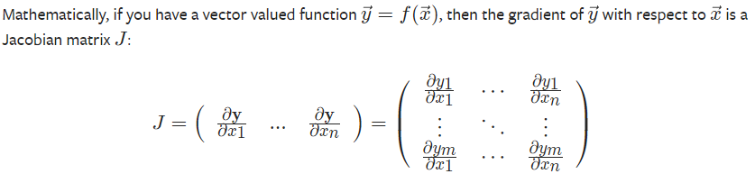
而autograd也可以用来计算雅各比行列式。

（三）计算图#

计算图是autograd的一种计算方法，称之为directed acyclic graph，在DAG中，叶子是输入张量，根是输出张量，通过追踪计算图的叶子到根，我们可以自动计算出梯度，使用链式法则。

前向传播中，autograd同时做两件事情：

• 运行必要的计算操作
• 保持梯度函数的操作，在DAG中

后向传播当.backward()被调用在DAG的根上，autograd则：

• 计算梯度的每个.grad_fn
• 加快张量的.grad属性计算
• 使用链式法则，传播给所连的叶子张量

DAG记录了每个张量的操作，当其requires_grad标志位设置为True，反之，将不会记录。在NN中，参数不更新叫做冻结参数（frozen parameters），如果你事先直到不需要梯度更新参数，这将是有用的。

from torch import nn, optim

model = torchvision.models.resnet18(pretrained=True)

# Freeze all the parameters in the network
for param in model.parameters():
    param.requires_grad = False

二、NEURAL NETWORKS#

一个典型的神经网络训练过程：

• 定义NN（一些可以学习的参数）
• 迭代输入的数据集
• 计算损失
• 运用后向传播和梯度
• 更新权重，一般简单的运用公式：weight = weight - learning_rate * gradient

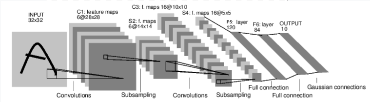
(一)定义网络#

class Net(nn.Module):

    def __init__(self):
        super(Net, self).__init__()
        # 1 input image channel, 6 output channels, 5x5 square convolution
        # kernel
        self.conv1 = nn.Conv2d(1, 6, 5)
        self.conv2 = nn.Conv2d(6, 16, 5)
        # an affine operation: y = Wx + b
        self.fc1 = nn.Linear(16 * 5 * 5, 120)  # 5*5 from image dimension
        self.fc2 = nn.Linear(120, 84)
        self.fc3 = nn.Linear(84, 10)

    def forward(self, x):
        # Max pooling over a (2, 2) window
        x = F.max_pool2d(F.relu(self.conv1(x)), (2, 2))
        # If the size is a square, you can specify with a single number
        x = F.max_pool2d(F.relu(self.conv2(x)), 2)
        x = torch.flatten(x, 1) # flatten all dimensions except the batch dimension
        x = F.relu(self.fc1(x))
        x = F.relu(self.fc2(x))
        x = self.fc3(x)
        return x


net = Net()
print(net)

>>>Net(
  (conv1): Conv2d(1, 6, kernel_size=(5, 5), stride=(1, 1))
  (conv2): Conv2d(6, 16, kernel_size=(5, 5), stride=(1, 1))
  (fc1): Linear(in_features=400, out_features=120, bias=True)
  (fc2): Linear(in_features=120, out_features=84, bias=True)
  (fc3): Linear(in_features=84, out_features=10, bias=True)
)

forward必须被定义，但是backward函数不需要，因为已经被自动定义。forward可以被用于任何张量操作。

Note：

torch.nn仅支持mini-batches。nn.Conv2d将喂入一个4dimension的张量，如nSamples x nChannels x Height x Width。如果是一个单个样本，使用input.unsqueeze(0)去增加一个虚拟batch维度。

Recap：

• torch.Tensor是一个多维向量，支持autograd

• nn.Module neural network模型，转化参数类型，可以移步到GPU去计算

• nn.Parameter 一种张量，可以自动地注册

• autograd.Function实现了autograd操作的前后传播定义，每一个张量操作创造至少一个Function节点，以此链接特殊的函数，这个特殊的函数创建了一个张量，并且编码了它的生命记录

（二）损失函数#

损失函数需要输出和目标值作为一对输入，并且计算他们俩之间的差距。

output = net(input)
target = torch.randn(10)  # a dummy target, for example
target = target.view(1, -1)  # make it the same shape as output
criterion = nn.MSELoss()

loss = criterion(output, target)
print(loss)

>>>
tensor(0.6493, grad_fn=<MseLossBackward0>)

如果我们跟随Loss在后向传播方向，使用Loss的.grad_fn，可以看到计算图。

input -> conv2d -> relu -> maxpool2d -> conv2d -> relu -> maxpool2d
      -> flatten -> linear -> relu -> linear -> relu -> linear
      -> MSELoss
      -> loss

(三)权重更新#

最简单的随机梯度下降（SGD），更新方法：

weight = weight - learning_rate * gradient

运用代码：

learning_rate = 0.01
for f in net.parameters():
    f.data.sub_(f.grad.data * learning_rate)

更多的更新方法在包torch.optim中。

三、CIFAR-10训练#

import torch
from torch import nn
from torch.utils.data import DataLoader
from torch.utils.tensorboard import SummaryWriter
from torchvision import datasets
from torchvision.transforms import ToTensor

torch.manual_seed(1)

# hyper parameters
Epoch = 10
Batch_size = 64
Learning_rate = 0.001

# Download training data from open datasets.
training_data = datasets.FashionMNIST(
    root="data",
    train=True,
    download=True,
    transform=ToTensor(),
)

# Download test data from open datasets.
test_data = datasets.FashionMNIST(
    root="data",
    train=False,
    download=True,
    transform=ToTensor(),
)

# Create data loaders.
train_dataloader = DataLoader(training_data, batch_size=Batch_size)
test_dataloader = DataLoader(test_data, batch_size=Batch_size)

for X, y in test_dataloader:
    print(f"Shape of X [N, C, H, W]: {X.shape}")
    print(f"Shape of y: {y.shape} {y.dtype}")
    break

# Get cpu or gpu device for training.
device = "cuda" if torch.cuda.is_available() else "cpu"
print(f"Using {device} device")


class CNN(nn.Module):
    def __init__(self):
        super(CNN, self).__init__()
        self.conv1 = nn.Sequential(  # input shape (1,28,28)
            nn.Conv2d(in_channels=1,  # input height
                      out_channels=16,  # n_filter
                      kernel_size=5,  # filter size
                      stride=1,  # filter step
                      padding=2  # con2d出来的图片大小不变
                      ),  # output shape (16,28,28)
            nn.ReLU(),
            nn.MaxPool2d(kernel_size=2)  # 2x2采样，output shape (16,14,14)

        )
        self.conv2 = nn.Sequential(nn.Conv2d(16, 32, 5, 1, 2),  # output shape (32,7,7)
                                   nn.ReLU(),
                                   nn.MaxPool2d(2))
        self.out = nn.Linear(32 * 7 * 7, 10)

    def forward(self, x):
        x = self.conv1(x)
        x = self.conv2(x)
        x = x.view(x.size(0), -1)  # flat (batch_size, 32*7*7)
        output = self.out(x)
        return output


cnn = CNN().to(device)
print(cnn)

# optimizer
optimizer = torch.optim.Adam(cnn.parameters(), lr=Learning_rate)

# loss_fun
loss_func = nn.CrossEntropyLoss()

write = SummaryWriter('logs')

def train(dataloader, cnn, loss_fn, optimizer):
    size = len(dataloader.dataset)
    cnn.train()
    for batch, (X, y) in enumerate(dataloader):
        X, y = X.to(device), y.to(device)

        # Compute prediction error
        pred = cnn(X)
        loss = loss_fn(pred, y)

        # Backpropagation
        optimizer.zero_grad()
        loss.backward()
        optimizer.step()

        write.add_scalar("train_loss",loss.item())
        if batch % 100 == 0:
            loss, current = loss.item(), batch * len(X)
            print(f"loss: {loss:>7f}  [{current:>5d}/{size:>5d}]")


def test(dataloader, cnn, loss_fn):
    size = len(dataloader.dataset)
    num_batches = len(dataloader)
    cnn.eval()
    test_loss, correct = 0, 0
    with torch.no_grad():
        for X, y in dataloader:
            X, y = X.to(device), y.to(device)
            pred = cnn(X)
            test_loss += loss_fn(pred, y).item()
            correct += (pred.argmax(1) == y).type(torch.float).sum().item()
    test_loss /= num_batches
    correct /= size
    print(f"Test Error: \n Accuracy: {(100*correct):>0.1f}%, Avg loss: {test_loss:>8f} \n")


print("------start training------")

for epoch in range(Epoch):
    print(f"Epoch {epoch + 1}\n-------------------------------")
    train(train_dataloader, cnn, loss_func, optimizer)
    test(test_dataloader, cnn, loss_func)

print("Done!")

out:

Shape of X [N, C, H, W]: torch.Size([64, 1, 28, 28])
Shape of y: torch.Size([64]) torch.int64
Using cuda device
CNN(
  (conv1): Sequential(
    (0): Conv2d(1, 16, kernel_size=(5, 5), stride=(1, 1), padding=(2, 2))
    (1): ReLU()
    (2): MaxPool2d(kernel_size=2, stride=2, padding=0, dilation=1, ceil_mode=False)
  )
  (conv2): Sequential(
    (0): Conv2d(16, 32, kernel_size=(5, 5), stride=(1, 1), padding=(2, 2))
    (1): ReLU()
    (2): MaxPool2d(kernel_size=2, stride=2, padding=0, dilation=1, ceil_mode=False)
  )
  (out): Linear(in_features=1568, out_features=10, bias=True)
)
------start training------
Epoch 1
-------------------------------
loss: 2.307641  [    0/60000]
loss: 0.737086  [ 6400/60000]
loss: 0.368927  [12800/60000]
loss: 0.530034  [19200/60000]
loss: 0.556181  [25600/60000]
loss: 0.511927  [32000/60000]
loss: 0.382789  [38400/60000]
loss: 0.543811  [44800/60000]
loss: 0.516559  [51200/60000]
loss: 0.427986  [57600/60000]
Test Error: 
 Accuracy: 85.4%, Avg loss: 0.404072 

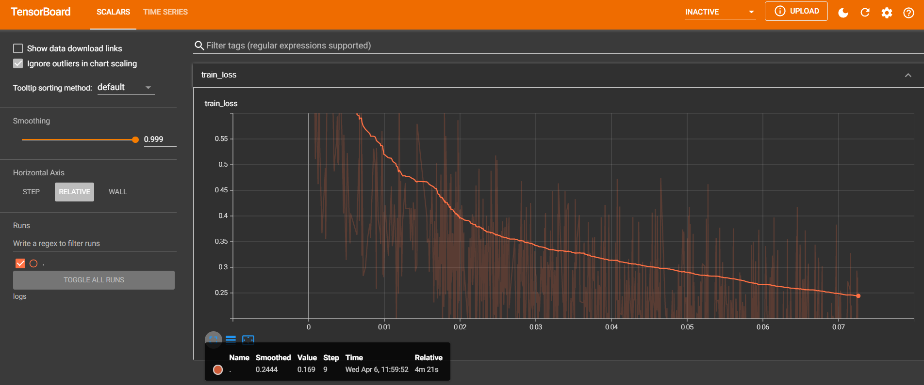
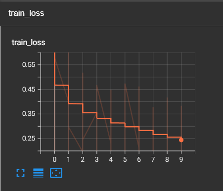
运行后在cmd输入以下命令查看训练状态：

tensorboard --logdir=logs --port=8080