
6D姿态估计从0单排——看论文的小鸡篇——A Novel Representation of Parts for Accurate 3D Object Detection and Tracking in Monocular Images
这个可以算我最长的一片笔记。。因为大部分的文字描述都是和公式做法密切相关。这个方法就是通过2个CNN模型,一个预测图片patch所属模型的部分part的control point,另一个预测part中心的reprojection,然后利用雅可比行列式和Using a single Gaussian Pose Prior中介绍的公式来迭代得到使得模型预测的reprojection和control point中心距离最小的pose,然后在经过训练的线性回归分类器检测选出来最好的pose,并且每帧的pose都会作为下一帧的先验
使用CNN来估计2D图像中的关键点位置,而且不只是2D,这篇文章的输入要求是灰度图
Our key idea is to then predict the 3D pose of each part in the form of the 2D projections of a few control points. Even though part of the object is visible, it can predict the 3D pose very accurate.
a depth sensor, which would fail on metallic objects or outdoor scenes
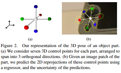
we therefore propose to represent the pose of each part by the 2D reprojections of a small set of 3D control points. The control points are only "virtual", and do not have to correspond to specific image features. We show that a CNN can predict the locations of these reprojections very accurate, and can also be used to predict the uncertainty of these location estimates.
Given an input image, we run a detector to obtain a few hypotheses on the image locations of each part. We also use a CNN for this task. We then predict the reprojections of the control points by applying a specific CNN to each hypothesis. This gives us a set of 3D-2D correspondences, some of which may be erroneous, but from which we can compute the 3D pose of the target object.
Given an input grayscale image2, we want to estimate the 3D pose \(p\) of a calibrated projective camera with respect to a known rigid object. We assume that we are given a 3D
model of the object and a set of manually labelled parts (in the test, less than 4) on the object. We currently select the parts by hand.
- Representing the Part Poses our solution is based on 3D control points. We directly predict the 3D locations of the 3D Control Points in the camera reference system: This makes combining the poses simpler, as this only involves computing the rigid motion between two sets of 3D points. This representation is not translation invariant. So we propose to represent the part pose as the 2D reprojections of a set of 3D control points. This representation is translation invariant and can combine the poses of an arbitrary number of parts by grouping all reprojections and solving a PnP problem. We used 7 control points for each part spanning 3 orthogonal directions.
- Detecting the Parts
![]()
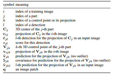
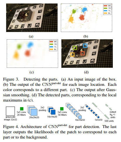
we use a set of registered training images of the target object under different poses and lighting to learn to detect the parts and predict their control points. Training data : \(T = \{ (I_i, \{c_{ij}\}_j, \{v_{ijk}\}_{jk}) \}\) where \(I_i\) denotes the \(i\)th training image. We train the CNN to detect the parts. The input to this CNN is a \(32\times32\) image patch \(q\), its output consists of the likelihoods \(P(J = j | q)\) of the patch to correspond to one of the \(N_P\)(num of the parts) parts. We train the CNN with patches randomly extracted around the centers \(c_{ij}\) of the parts in images \(I_i\) and patches extracted from the background, and by optimizing the negative log-likelihood over the parameters \(w\) of the CNN:
\(\hat{w}=\arg\min\sum^{N_p}_{j=0}\sum_{q\in T_j}-\log softmax(CNN^{part-det}_w(q)[j])\)
where \(T_j\) is a training set made of image patches centered on part \(j\) and \(T_0\) is a training set made of image patches from the background, \(CNN^{part-det}_w(q)\) is \(N_p+1\)-vector and \([j]\) means the \(j\)-th coordinate of cector \(CNN^{part-det}_w(q)\). At run time, we obtain the clusters of large values for the likelihood of each part around the centers of the parts. We apply a smoothing Gaussian filter on the output, and retain only the local maximums of these values as candidates for the locations of the parts. The result of this step is, for each part \(j\), a set \(S_j = \{(\hat{c}_{jl},s_{jl})\}_l\) of 2D location candidate \(\hat{c}_{jl}\) for the part together with a score \(s_{jl}\) that is the value of the local maxima returned by the CNN. We typically get up to 4 detections for each part in a given input image. - Predicting the Reprojections of the Control Points and their Uncertainty
![]()
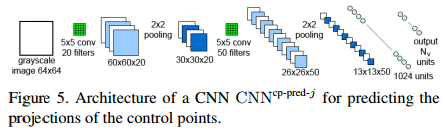
Once the parts are detected, we apply a second CNN to the patches centered on the candidates \(\hat{c}_{jl}\) to predict the projections of the control points for these candidates. Each part has its specific CNN. \(N_V\) is the number of control points of the part.We train each of these CNNs during an offline stage by simply minimizing over the parameters \(w\) of the CNN the squared loss of the predictions:
\(\hat{w}=\arg\min\sum_{(q,w)\in V_j}\left\|w-CNN^{cp-preb-j}_w(q)\right\|^2)\)
where \(V_j\) is a training set of image patches \(q\) centered on part \(j\) and the corresponding 2D locations of the control points concatenated in a \((2N_V)\)-vector \(w\), and \(CNN^{cp-preb-j}_w(q)\) is the prediction for these locations made by CNN specific for part \(j\), given parch \(q\) as input. In addition, we estimate the 2D uncertainty for the predictions, by propagating the image noise through the CNN that predicts the control point projections. At last, the matrix: \(S_V = J_{\hat{c}}(\sigma I)J_{\hat{c}}^T\), where \(\sigma\) is the standard deviation of the image noise assumed to be Gaussian and affected each image pixel independently. \(J_{\hat{c}}\) the Jacobian of the function computed by the CNN
Estimating the Object Pose
We assume that we are given a prior on the pose p, in the form of a Mixture-of-Gaussians \(\{(\bar{p_m}, S_m)\}\). This prior is very general, and allows us to define the normal action range of the camera. Moreover, the pose computed for the previous frames can be easily incorporated within this framework to exploit temporal consistency.
- Using a single Gaussian Pose Prior
The pose \(\hat{p}\) can be estimated as the minimizer of: \(\frac{1}{N_p}\sum_{j,k}dist^2(S_{jk}, \Gamma_p(V_{jk}),\hat{v}_{jk}) + (p - \bar{p_0})^TS^{-1}_0(p - \bar{p_0}))\), where the sum is over all the control points of all the parts and \(\Gamma_p(V)\) is the 2D projection of \(V\) under pose \(p\). \(\hat{v}_{jk}\) is the projection of control point \(V_{jk}\) and \(S_{jk}\) its uncertainty estimated as explained. \(dist^2(S, v_1, v_2) = (v_1 - v_2)^TS^{-1}(v_1 - v_2)\). \(F(p)\) is minimized using the Gauss-Newton algorithm initialized with \(p0\). - Robust detection of parts
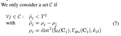
we rank the candidates according to their score \(s_{jl}\), keep the best four candidates for each part and greedily examine the possible sets \(C\) of correspondences between a part and the candidate detections.
![]()
where \(T=40\), \(\hat{S}_0(C_j)=JS_0J^T\), with \(J\) the jacobian of \(\Gamma_{p_0}(C_j)\) is the covariance of the projection \(\Gamma_{p_0}(C_j)\) of \(C_j\), and \(p_{\hat{j}}\) is a random candidate of the set. If \(C\) passes, we compute the average distance \(\bar{p} = \frac{1}{|C|}\sum_j\tilde{p_j}\) of its points. We keep the \(N_C\)(we set 4) sets with the lowest average distance. we run the Gauss-Newton optimization using each \(C\) to obtain a pose estimate. - Using a Mixture-of-Gaussians for the Pose Prior
![]()
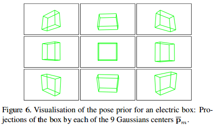
In practice, the prior for the pose is in the form of a Mixture-of-Gaussians \(\{(\bar{p_m},\sum_m)\}\) with \(M=9\) components. We apply the method described above to each component, and obtain \(M N_C\) possible pose estimates.
To finally identify the best pose estimate, we evaluate each pose, employing a weighted sum of several cues: the angle between the quaternions for pose and the corresponding \(\bar{p_m}\) prior; the average reprojection error of the set of control points C according to pose; the correlation between the object contours amd edges after projection by pose. we train a simple linear regressor on the training video sequences to predict the Euclidean distance between pose and the groundtruth. We add to the initial prior the estimated pose and its covariance as part of the pose prior for the next frame.

 浙公网安备 33010602011771号