6D姿态估计从0单排——看论文的小鸡篇——Multimodal Templates for Real-Time Detection of Texture-less Objects in Heavily Cluttered Scenes
Multimodal Templates for Real-Time Detection of Texture-less Objects in Heavily Cluttered Scenes
6D姿态估计里面的linemod方法的来源,作者也是慕尼黑工业大学的大牛。
基于linemod
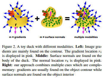
For such time-critical applications, template matching is an attractive solution because new objects can be easily learned online; more particularly to , which consider only images and their gradients to detect objects. As such, they work even when the objects is not textured enough to use feature point techniques.
- Similarity Measure
![]()
reference images \(\{O_m\}_{m\in M}\), object from a set \(M\) of modalities.
A template \(\tau = (\{O_m\}_{m\in M}, P)\), \(P\) is list of pairs \((r, m)\), \(r\) is locations of discriminant feature in modality \(m\).
Each template is created by extracting for each modality a small set of its most discriminant features from the corresponding reference image and by storing their locations
Our similarity measure is a generalization of the measure which is robust to small translations and deformations. It can be formalized as
\(\varepsilon(\{I_m\}_{m\in M}, \tau, c) = \sum_{(r,m)\in P}(\max_{t\in R(c+r)} f_m(O_m(r), I_m(t)))\), \(R(c+r) = [c+r-\frac{T}{2}, c+r+\frac{T}{2}]\times[c+r-\frac{T}{2}, c+r+\frac{T}{2}]\) defines the neighborhood of size \(T\) centered on location \(c+r\) in the input image \(I_m\) and the function \(f_m(O_m(r), I_m(t))\) computes the similarity score for modality \(m\) between the reference image at location \(r\) and the input image at location \(t\). - Efficient Computation
quantize the input data for each modality into a small number of \(n_0\), which allows us to "spread" the data around their locations to obtain a robust representation \(J_m\) for each modality. use a lookup table \(\tau_{i,m}\) for each modality and for each of \(n_0\) quantized values, computed offline as: \(\tau_{i,m}[L_m] = \max_{l\in L_m}\left|f_m(i,l)\right|\), \(i\) is the index of the quantized value of modality \(m\), \(L_m\) is list of values of a special modality \(m\) appearing in a local neighborhood of a value \(i\), use \(L_m\) as index to the element in the lookup table. So for each quantized value of ont modality \(m\) with index \(i\), we can compute the response at each location \(c\) of the response map \(S_{i,m}\) as : \(S_{i,m}(c) = \tau_{i,m}[J_m(c)]\). Finally, we can get: \(\varepsilon(\{I_m\}_{m\in M}, \tau, c) = \sum_{(r,m)\in P}S_{O_m(r),m}(c + r)\) - Modality Extraction
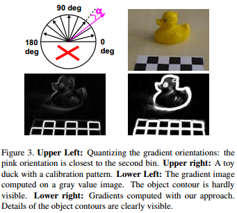
Image Cue: consider image gradients because they proved to be more discriminant than other forms of representations and tobust to illumination change and noise; Image gradients are often the only reliable image cue when it comes to texture-less objects; We compute the normalized gradients on each color channel of our input image separately and for each image location use the normalized gradient of
the channel whose magnitude is largest.
![]()
we compute the normalized gradient map \(I_G(x)\) at location with \(I_G(x) = \frac{\vartheta \hat{C}}{\vartheta x}\), where \(\hat{C}(x) = \arg\max_{C \in R,G,B}\left\|\frac{\vartheta C}{\vartheta x}\right\|\) and R,G,B are the RGB channels of corresponding color image. Similarity measure is \(f_G(O_G(r), I_G(t) = \left| O_G(r)^T I_G(t)\right|)\), where \(O_G(r)\) is the normalized gradient map of reference image at location \(r\) and \(I_G(t)\) the normalized gradient map of current image at location \(t\) respectively. In order to quantize the gradient map we omit the gradient direction, consider only the gradient orientation and divide the orientation space into n0 equal spacings. To make the quantization robust to noise, we assign to each location the gradient whose quantized orientation occurs most often in a 3 × 3 neighborhood.
Depth Cue:
![]()
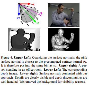
use quantized surface normals computed on a dense depth field for our template representation.
Around each pixel location x, we consider the first order Taylor expansion of the depth function \(D(x)\): \(D(x + dx) - D(x) = dx^T \nabla D + h.o.t\). This depth gradient corresponds to a 3D plane going through three points X, X1 and X2:
\(X = \vec{v(x)}D(x)\),
\(X1 = \vec{v}(x + [1, 0]^T)(D(x) + [1, 0]\nabla \hat{D})\),
\(X2 = \vec{v}(x + [0, 1]^T)(D(x) + [0, 1]\nabla \hat{D})\),
where \(\vec{v}(x)\) is the vector along the line of sight that goes through pixel \(x\) and is computed from the internal paramenters og the depth sensor. The normal to the surface at the 3D point that projects on x can be estimated as the normalized cross-product of \(X1 − X\) and \(X2 − X\). we ignore the contributions of pixels whose depth difference with the central pixel is above a threshold. Our similarity measure is then defined as the dot product of the normalized surface
normals: \(f_D(O_D(r), I_D(t) = O_D(r)^T I_D(t))\), where \(O_D(r)\) is the normalized surface normal map of the reference image at location \(r\) and \(I_D(t)\) the normalized surface normal map of the current image at location \(t\). we measure the angles between the computed normal and a set of precomputed vectors to quantize the normal directions into \(n_0\) bins.These vectors are arranged in a right circular cone shape originating from the peak of the cone pointing towards the camera. To make the quantization robust to noise, we assign to each location the quantized value that occurs most often in a 5 × 5 neighborhood.


 浙公网安备 33010602011771号