Signal Filters Design Based on Digital Signal Processing

Thoeries

I. Fourier Series Expansion Algorithm

We can utilize the Fourier Series to produce the analog signal with some frequency components. For any signal, its Fourier series expansion is defined as

$$x(t)=\frac{A_0}{2}+\sum _{n=1}^{\mathrm{\infty }}{A}_n\cos (n\mathrm{\Omega }t+{\phi }_n)$$

In the equation，$\frac{A_0}{2}$ represents the DC component, $A_1\cos (\mathrm{\Omega }t+{\phi }_1)$, represents the fundamental component of the signal, $A_n\cos (n\mathrm{\Omega }t+{\phi }_n)$ represents the nth harmonic component of the signal. Moreover, analog angular frequency $\mathrm{\Omega }=\frac{2\pi }{T}=2\pi f$.
Therefore, in this project we select three different frequency components, that is $f_1,f_2,f_3$, to synthesize the final required analog signal:

$$x(t)=\frac{A_0}{2}+A_1\cos (2\pi f_{1}t+{\phi }_1)+A_2\cos (2\times 2\pi f_{2}t+{\phi }_2)+A_3\cos (3\times 2\pi f_{3}t+{\phi }_3)$$

For simplicity, there we respectively select these values:

$A_0=0,A_1=1,A_2=1,A_3=1$ $${\phi }_1={\phi }_2={\phi }_3=0$$ Following above expression, we can get the generated analog signal: $$x(t)=\cos (2\pi f_{1}t)+\cos (4\pi f_{2}t)+\cos (6\pi f_{3}t)$$

II. Sample the Analog Signal

Time Domain Sampling Theorem

According to the time domain sampling theorem, the sampling frequency must be greater than twice the signal cutoff frequency.
Let's assume that the sampling frequency is $F_s$, and the generated analog signal frequency satisfies: $F_1<F_2<F_3$, so the signal cutoff frequency is $F_c=F_3$. The sampling theorem is formally expressed as:

$$F_s>2F_c$$

In this experiment，we respectively selected $F_1=10Hz,F_2=20Hz,F_3=30Hz$ to produce analog signal. So we can get the period and cutoff frequency of sampled signal:

$$T_c=\frac{1}{F_1}=0.1s,F_c=F_3=30Hz$$

Time-domain Window

For periodic continuous signals, we intercept at integer multiples of the period to obtain a sequence for spectrum analysis.

$$T_p=N\ast T_c,N\in Z^{+}$$

Sampling Frequency

For a specific sampling frequency, we can get the sampling period $T_s$, and the number of sampling points $N$:

$$T_s=\frac{1}{F_s},N=T_p\ast F_c$$

Therefore, we use sampling frequency of $F_s=90Hz,F_s=60Hz,F_s=40Hz$ to get time-domain signals.

Spectral Resolution

Spectral resolution is defined as the minimum separation between two signals of different frequencies:

$$\mathrm{\Delta }f=\frac{F_s}{N}=\frac{1}{N{T}_s}=\frac{1}{T_p}$$

III. Spectral Analysis

In this section, we will analyse the Amplitude-Frequency Characteristics and Phase-Frequency Characteristics of the sampled signal.

Convert to Frequency

When analysing the spectral, we need to convert the $0\sim N-1$ to frequency sequence:

$$f_k=k\ast \frac{F_s}{N},k=0,1,...N-1$$

Convert to Real Amplitude

After we apply Discrete Fourier Transform to the sampled signal, the frequency-domain signal is complex-valued. And due to the time-domain signal is real-valued, the the frequency-domain signal is conjugate symmetric:

$$X(k)=X^{\ast }(N-k),k=0,1,...N-1$$

For complex values, that means its real part is even symmetric about the middle point, and its imaginary part is odd symmetric about the middle point. This will be showed in the following figures.

Experiments

Experiment I: $T_p=3T_c,F_s=90$Hz

• Samping Frequency $F_s=3F_c(F_s>2F_c)$
  We use the sampling frequency of $F_s=90$Hz under the condition of $T_p=3T_c$.
  
  
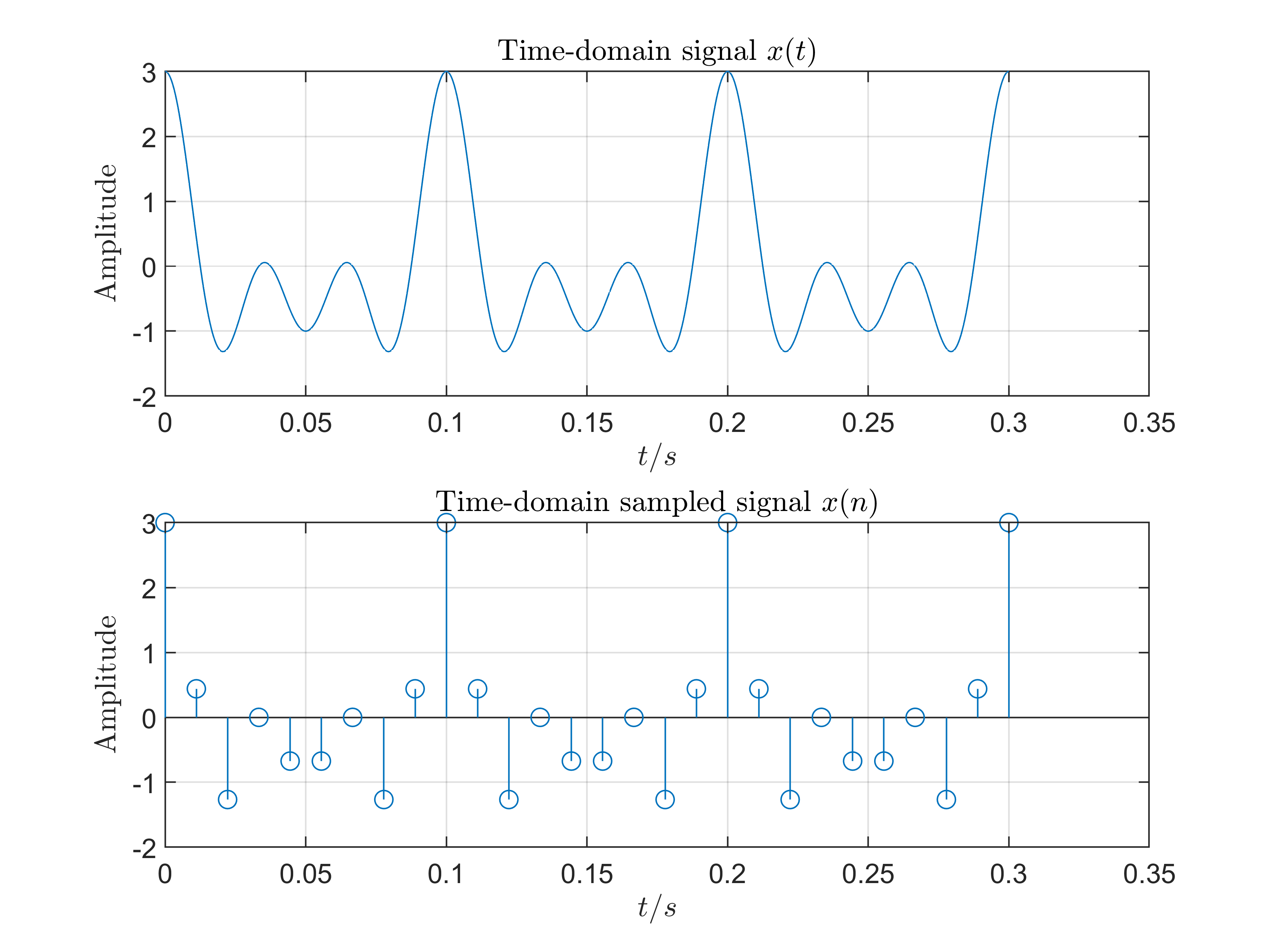
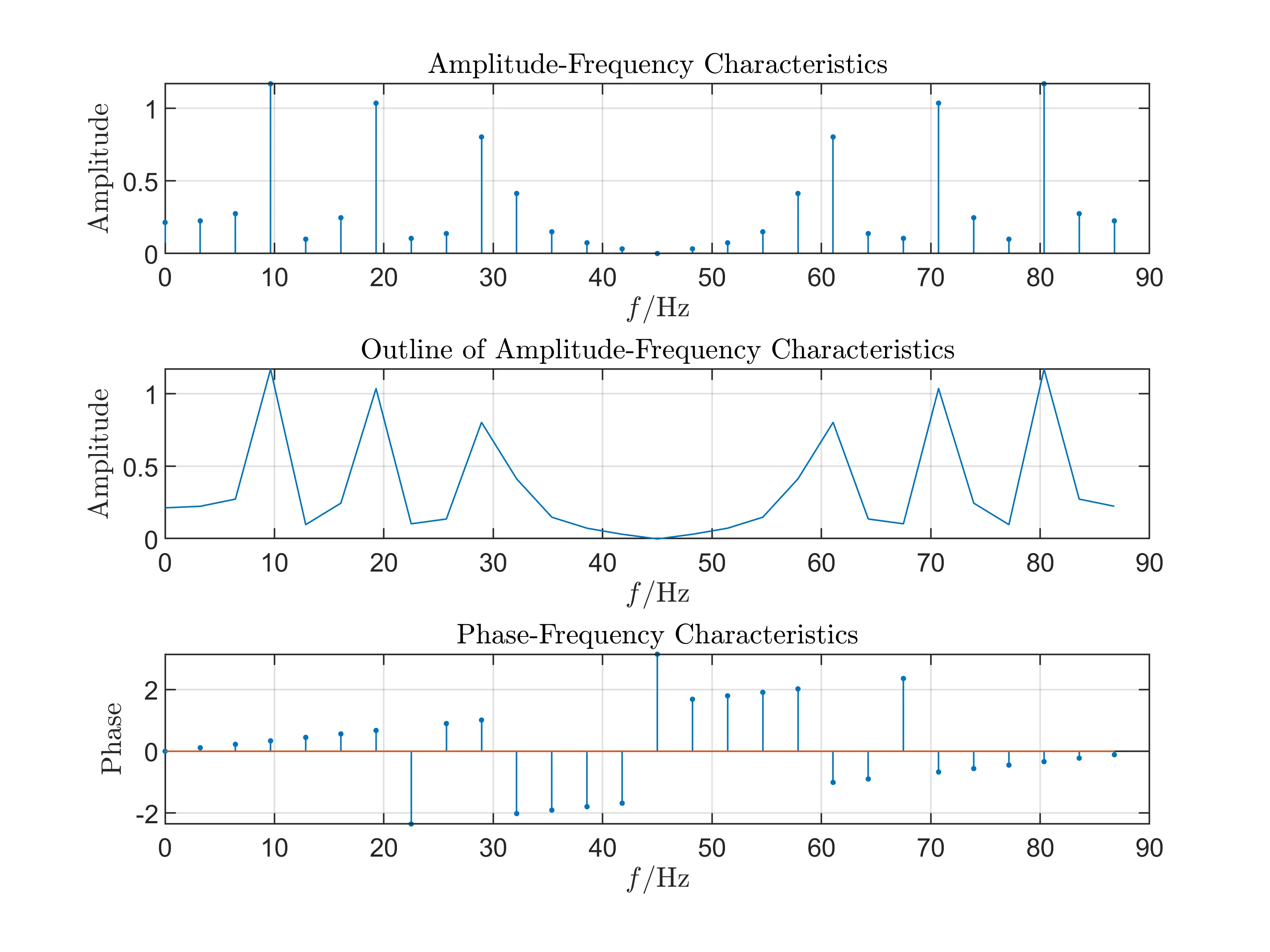
• Conclusions
  The sampling frequency satisfies the Time Domain Sampling Theorem so we can see there is no overlap in frequency domain about the amplitude-frequency characteristic. And when $f=10$Hz, $f=20$Hz, $f=30$Hz, we can get the amplitude very close to $1$ which is us defined in analop signal.

Experiment II: $T_p=3T_c,F_s=60$Hz

• Samping Frequency $F_s=2F_c(F_s=2F_c)$
  We use the sampling frequency of $F_s=60$Hz under the condition of $T_p=3T_c$.
  
  
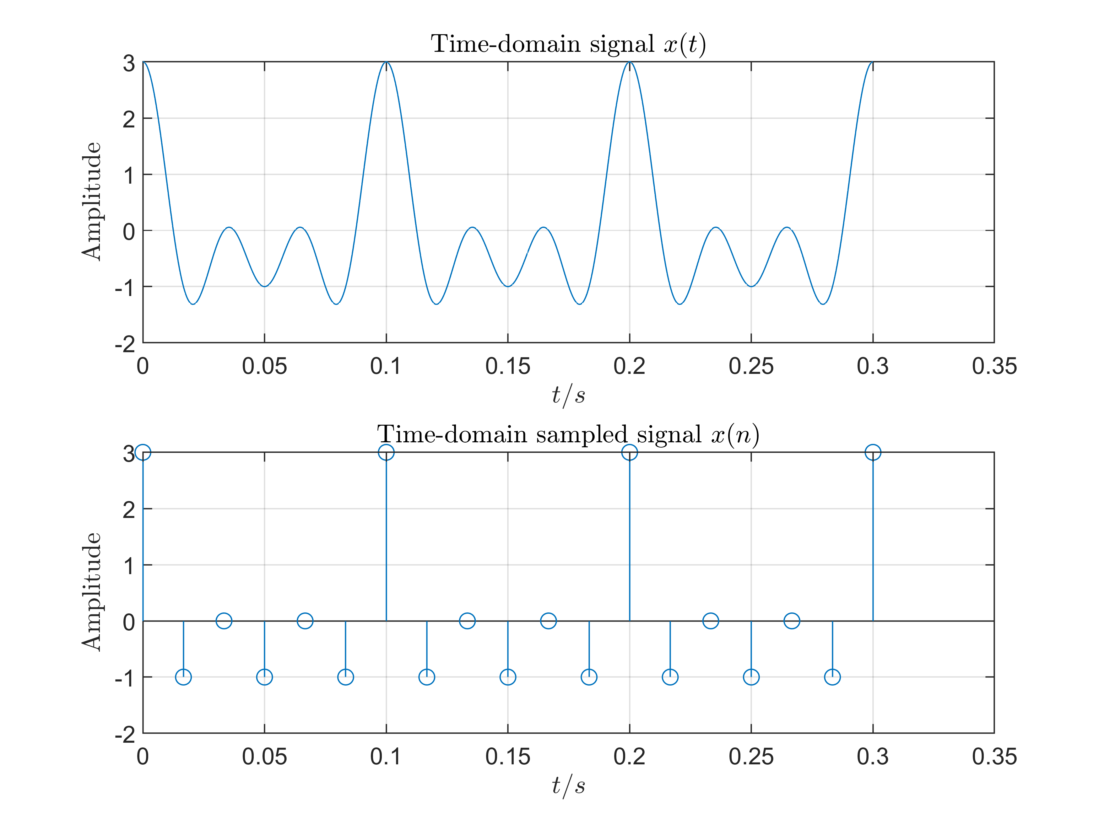
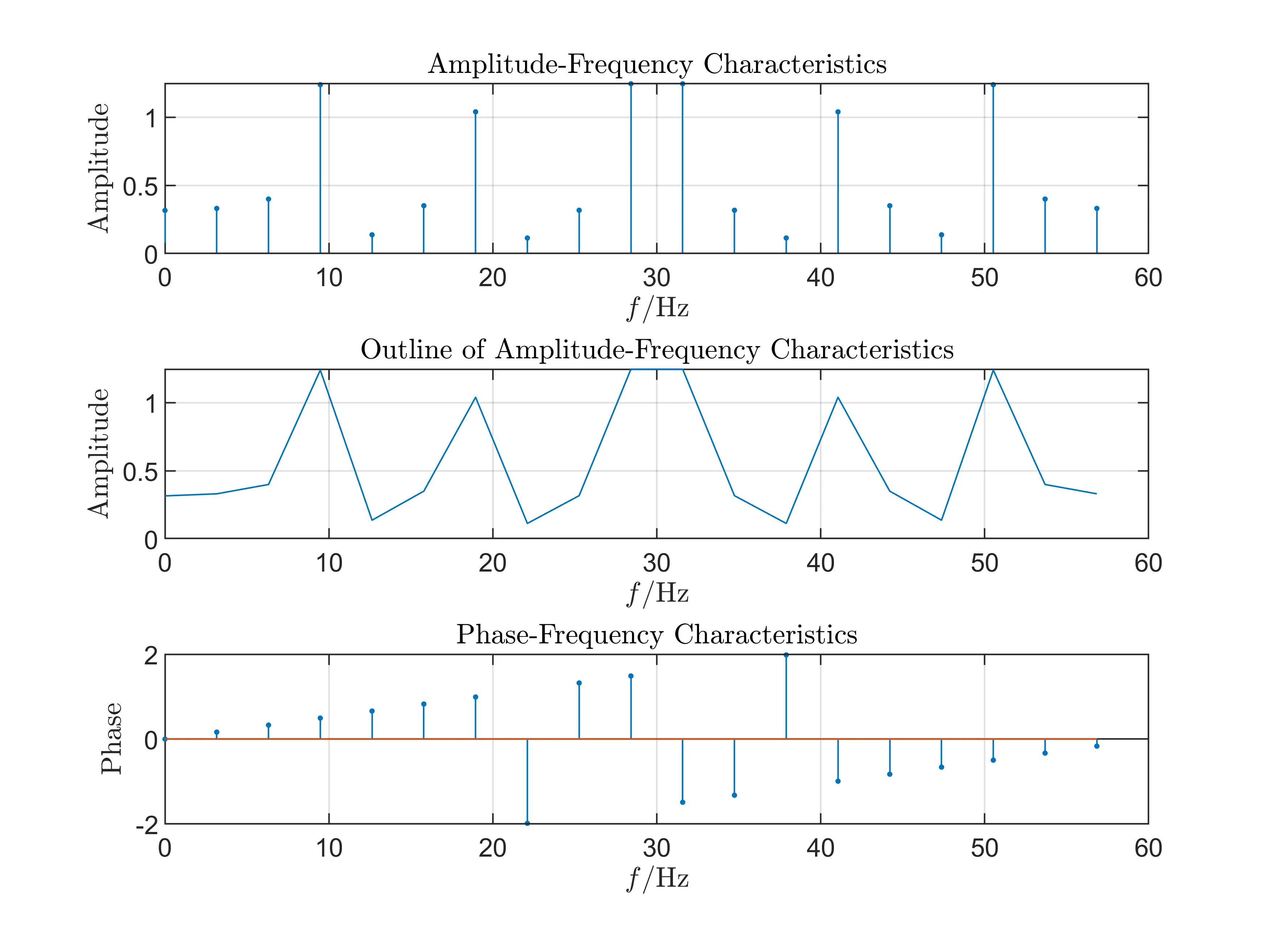
• Conclusions
  The sampling frequency equals the threhold of Time Domain Sampling Theorem so we can easily see that it will just become overlapping in frequency domain. And when $f=30$Hz that is also $F_s/2$ point, we can get this point very close to its symmetric frequency point.

Experiment III: $T_p=3T_c,F_s=40$Hz

• Samping Frequency $F_s=\frac{4}{3}{F}_c(F_s<2F_c)$
  We use the sampling frequency of $F_s=40$Hz under the condition of $T_p=3T_c$.
  
  
• Conclusions
  The sampling frequency do not equal the Time Domain Sampling Theorem so we can obviously see that it has discarded the third frequency $f=30$Hz, which is caused by overlapping in frequency domain.

Note: in order to clearly analyse spectral of sampled signal, we also select the Time-domain Window of $T_p=50T_c$ to conduct experiments.

Results

Experiment I: $F_s=40$Hz

Codes

%% Project Introduction:
%   This project is developed to design some signal filters based on digital
% signal processing.
clear, close all;
%% Produce and sample digital signal
f1 = 10;
f2 = 20;
f3 = 30;    % so the fc = f3 = 30Hz
Np = 50;          % number of periods for time-domain window
%% Experiment 1 (Choosing samling frequency fs = 3fc (fs > 2fs))
fs1 = 90;          % sampling frequency
xn1 = ProduceSamplingSignal(f1, f2, f3, fs1, Np, 'Sampling Analog Signal(fs = 3fc)');
DFTAnalysis(xn1, fs1, 'Frequency Response Characteristics(fs = 3fc)');

%% Experiment 2 (Choosing samling frequency fs = 2fc)
fs2 = 60;          % sampling frequency
xn2 = ProduceSamplingSignal(f1, f2, f3, fs2, Np, 'Sampling Analog Signal(fs = 2fc)');
DFTAnalysis(xn2, fs2, 'Frequency Response Characteristics(fs = 2fc)');

%% Experiment 3 (Choosing samling frequency fs < 2fc)
fs3 = 40;          % sampling frequency
xn3 = ProduceSamplingSignal(f1, f2, f3, fs3, Np, 'Sampling Analog Signal(fs < 2fc)');
DFTAnalysis(xn3, fs3, 'Frequency Response Characteristics(fs < 2fc)');

%% Experiment Description
% Experiment 4-7: Design a digital filter respectively with band pass, high
% pass, low pass, band stop based on ellipord.
%% Experiment 4: Design a digital filter with band pass using ellipord
fpl = 15; fpu=25; fsl=13; fsu=28;
rp = 1;             
rs = 40;
ellipBandPass(fpl, fpu, fsl, fsu, rp, rs, xn1, fs1, f1, Np, 'Digital Filter With Band Pass Using Ellipord(fs = 3fc)');
ellipBandPass(fpl, fpu, fsl, fsu, rp, rs, xn2, fs2, f1, Np, 'Digital Filter With Band Pass Using Ellipord(fs = 2fc)');
ellipBandPass(8, 10, 6, 12, rp, rs, xn3, fs3, f1, Np, 'Digital Filter With Band Pass Using Ellipord(fs < 2fc)');

%% Experiment 5: Design a digital filter with high pass using ellipord
fpz = 16; fsz = 13;
rp = 1;             
rs = 40;
ellipHighPass(fpz, fsz, rp, rs, xn1, fs1, f1, Np, 'Digital Filter With High Pass Using Ellipord(fs = 3fc)');
ellipHighPass(fpz, fsz, rp, rs, xn2, fs2, f1, Np, 'Digital Filter With High Pass Using Ellipord(fs = 2fc)');
ellipHighPass(15, 12, rp, rs, xn3, fs3, f1, Np, 'Digital Filter With High Pass Using Ellipord(fs < 2fc)');

%% Experiment 6: Design a digital filter with low pass using ellipord
fpz = 23; fsz=28; 
rp = 1;             
rs = 40;
ellipLowPass(fpz, fsz, rp, rs, xn1, fs1, f1, Np, 'Digital Filter With Low Pass Using Ellipord(fs = 3fc)');
ellipLowPass(fpz, fsz, rp, rs, xn2, fs2, f1, Np, 'Digital Filter With Low Pass Using Ellipord(fs = 2fc)');
ellipLowPass(12, 15, rp, rs, xn3, fs3, f1, Np, 'Digital Filter With Low Pass Using Ellipord(fs < 2fc)');

%% Experiment 7: Design a digital filter with band stop using ellipord
fpl = 15; fpu=25; fsl=17; fsu=22;
rp = 1;             
rs = 40;
ellipBandStop(fpl, fpu, fsl, fsu, rp, rs, xn1, fs1, f1, Np, 'Digital Filter With Band Stop Using Ellipord(fs = 3fc)');
ellipBandStop(fpl, fpu, fsl, fsu, rp, rs, xn2, fs2, f1, Np, 'Digital Filter With Band Stop Using Ellipord(fs = 2fc)');
ellipBandStop(5, 17, 8, 12, rp, rs, xn3, fs3, f1, Np, 'Digital Filter With Band Stop Using Ellipord(fs < 2fc)');

%% Experiment Description
% Experiment 8-11: Design a digital filter respectively with high pass, low
% pass, band pass, band stop based on hamming window.
%% Experiment 8: Design a digital filter with high pass using hamming window
fpz = 16; fsz = 13;
firlHighPass(fpz, fsz, xn1, fs1, f1, Np, 'Digital Filter With High Pass Using Hamming Window(fs = 3fc)');
firlHighPass(fpz, fsz, xn2, fs2, f1, Np, 'Digital Filter With High Pass Using Hamming Window(fs = 2fc)');
firlHighPass(15, 12, xn3, fs3, f1, Np, 'Digital Filter With High Pass Using Hamming Window(fs < 2fc)');
%% Experiment 9: Design a digital filter with low pass using hamming window
fpz = 23; fsz = 28;
firlLowPass(fpz, fsz, xn1, fs1, f1, Np, 'Digital Filter With Low Pass Using Hamming Window(fs = 3fc)');
firlLowPass(fpz, fsz, xn2, fs2, f1, Np, 'Digital Filter With Low Pass Using Hamming Window(fs = 2fc)');
firlLowPass(13, 17, xn3, fs3, f1, Np, 'Digital Filter With Low Pass Using Hamming Window(fs < 2fc)');
%% Experiment 10: Design a digital filter with band pass using hamming window
fpl = 15; fpu = 25;
firlBandPass(fpl, fpu, xn1, fs1, f1, Np, 'Digital Filter With Band Pass Using Hamming Window(fs = 3fc)');
firlBandPass(fpl, fpu, xn2, fs2, f1, Np, 'Digital Filter With Band Pass Using Hamming Window(fs = 2fc)');
firlBandPass(7, 15, xn3, fs3, f1, Np, 'Digital Filter With Band Pass Using Hamming Window(fs < 2fc)');
%% Experiment 11: Design a digital filter with band stop using hamming window
fsl = 15; fsu = 25;
firlBandStop(fsl, fsu, xn1, fs1, f1, Np, 'Digital Filter With Band Stop Using Hamming Window(fs = 3fc)');
firlBandStop(fsl, fsu, xn2, fs2, f1, Np, 'Digital Filter With Band Stop Using Hamming Window(fs = 2fc)');
firlBandStop(7, 15, xn3, fs3, f1, Np, 'Digital Filter With Band Band Stop Hamming Window(fs < 2fc)');

function xn = ProduceSamplingSignal(f1, f2, f3, fs, Np, Alltitle)
% Function Description: 
%        We want to make a digital signal composed of three frequency
%        components and sample the produced signal.
% Inputs: 
%        f1, f2, f3: means our selected frequency components, fs
%            represents the sampling frequency.
%        Np: means the number of periods.
% Outputs:
%        xn: represents the sampled signal.

    period = 1/f1;        % the period of analog signal(assuming f1 is the minimal)
    T = Np*period;         % sampling time-domain window(several periods)
    Ts = 1 / fs;          % sampling timestep
    t = 0: Ts : T;       % samping sequence of discrete sampling points
    % t = 0: 0.0001: T;     % analog time sequence

    % Step I: Produce digital signal
    xt = cos(2*pi*f1*t) + cos(2*pi*f2*t) + cos(2*pi*f3*t);
    % Step II: Sample produced signal
    xn = cos(2*pi*f1*t) + cos(2*pi*f2*t) + cos(2*pi*f3*t);

    % Step III: Visualize produced signal and sampled signal
    figure('Position', [210, 80, 950, 750]);
    subplot(2, 1, 1);
    plot(t, xt);
    title('Time-domain signal $x(t)$', 'Interpreter', 'latex', 'FontSize', 12);
    xlabel('$t/s$', 'Interpreter', 'latex', 'FontSize', 12);
    ylabel('Amplitude', 'Interpreter', 'latex', 'FontSize', 12);
    ylim([-2.5, 3.5]);
    grid on

    subplot(2, 1, 2);
    stem(t, xn);
    title('Time-domain sampled signal $x(n)$', 'Interpreter', 'latex', 'FontSize', 12);
    ylabel('Amplitude', 'Interpreter', 'latex', 'FontSize', 12);
    xlabel('$t/s$', 'Interpreter', 'latex', 'FontSize', 12);
    ylim([-2.5, 3.5]);
    grid on
    sgtitle(Alltitle, 'FontName', 'Times New Roman', 'FontSize', 14);
end

function DFTAnalysis(xn, fs, Alltitle)
% Function Description:
%       This function calculates the DFT[x(n)] and do spectral analysis.
% Inputs:
%       xn: digital discrete signal
%       fs: sampling frequency
% Outputs:
%       No return

    N = length(xn);    % number of sampling points
    df = fs / N;       % spectral resolution
    f1 = (0:N-1)*df;    % tranverse to the frequncy sequence
    f2 =  2*(0:N-1)/N;
    % DFT using FFT algorithm
    Xk = fft(xn, N);   
    % Tranverse to the real amplitude
    RM = 2*abs(Xk)/N;
    Angle = angle(Xk);

    figure('Position', [210, 80, 950, 750]);
    % Amplitude-Frequency Characteristics
    subplot(4,1,1);
    stem(f1, RM,'.');
    title('Amplitude-Frequency Characteristics', 'Interpreter', 'latex', 'FontSize', 12);
    xlabel('$f$/Hz', 'Interpreter', 'latex', 'FontSize', 12);
    ylabel('Amplitude', 'Interpreter', 'latex', 'FontSize', 12);
    grid on;
    
    % Phase-Frequency Characteristics
    subplot(4,1,2);
    stem(f1, Angle,'.'); 
    line([(N-1)*df, 0],[0,0]);
    title('Phase-Frequency Characteristics', 'Interpreter', 'latex', 'FontSize', 12);
    xlabel('$f$/Hz', 'Interpreter', 'latex', 'FontSize', 12);
    ylabel('Phase', 'Interpreter', 'latex', 'FontSize', 12);
    grid on;

    % Amplitude-Frequency Characteristics
    subplot(4,1,3);
    plot(f2, abs(Xk));
    title('Amplitude-Frequency Characteristics', 'Interpreter', 'latex', 'FontSize', 12);
    xlabel('\omega/\pi', 'FontSize', 12);
    ylabel('Amplitude', 'Interpreter', 'latex', 'FontSize', 12);
    grid on;
    
    % Phase-Frequency Characteristics
    subplot(4,1,4);
    plot(f2, Angle);
    title('Phase-Frequency Characteristics', 'Interpreter', 'latex', 'FontSize', 12);
    xlabel('\omega/\pi', 'FontSize', 12);
    ylabel('Phase', 'Interpreter', 'latex', 'FontSize', 12);
    ylim([-3.5, 3.5]);
    grid on;
    sgtitle(Alltitle, 'FontName', 'Times New Roman', 'FontSize', 14);
end

function ellipBandPass(fpl, fpu, fsl, fsu, rp, rs, x, fs, f1, Np, Alltitle)
    wp = [2*fpl/fs, 2*fpu/fs];
    ws = [2*fsl/fs, 2*fsu/fs];
    [N, wn] = ellipord(wp, ws, rp, rs);    % 获取阶数和截止频率
    [B, A] = ellip(N, rp, rs, wn, 'bandpass');         % 获得转移函数系数

    filter_bp_s = filter(B, A, x);
    X_bp_s = abs(fft(filter_bp_s));
    X_bp_s_angle = angle(fft(filter_bp_s));
    
    % plot the graphs    
    period = 1/f1;        % the period of analog signal(assuming f1 is the minimal)
    T = Np*period;         % sampling time-domain window(several periods)
    Ts = 1 / fs;          % sampling timestep
    t = 0: Ts : T;       % samping sequence of discrete sampling points
    N = length(x);    % number of sampling points
    f =  2*(0:N-1)/N;

    % 带通滤波器频谱特性
    figure('Position', [210, 80, 950, 750]);
    subplot(4,4,[1,2,5,6]);
    M = 512;
    wk = 0:pi/M:pi;
    Hz = freqz(B,A,wk);
    plot(wk/pi, 20*log10(abs(Hz)));
    xlabel('\omega/\pi', 'FontSize', 12);
    ylabel('$20lg|Hg(\omega)|$', 'Interpreter', 'latex', 'FontSize', 12);
    title('带通滤波器频谱特性');
    axis([0.2,0.9,-80,20]);set(gca,'Xtick',0:0.1:1,'Ytick',-80:20:20);
    grid on;

    subplot(4,4,[3,4,7,8]);
    plot(t, filter_bp_s);
    xlabel('t/s', 'Interpreter', 'latex', 'FontSize', 12);
    ylabel('Amplitude', 'Interpreter', 'latex', 'FontSize', 12);
    grid on;

    subplot(4,4,[9, 10, 11, 12]);
    plot(f, X_bp_s);
    title('带通滤波后频域幅度特性');
    ylabel('Amplitude', 'Interpreter', 'latex', 'FontSize', 12);
    grid on;

    subplot(4,4,[13, 14, 15, 16]);
    plot(f, X_bp_s_angle);
    title('带通滤波后频域相位特性');    
    xlabel('\omega/\pi', 'FontSize', 12);
    ylabel('Phase', 'Interpreter', 'latex', 'FontSize', 12);
    ylim([-3.5, 3.5]);
    grid on;
    sgtitle(Alltitle, 'FontName', 'Times New Roman', 'FontSize', 14);
end

function ellipHighPass(fpz, fsz, rp, rs, x, fs, f1, Np, Alltitle)
    wpz = 2*fpz/fs;
    wsz = 2*fsz/fs;
    [N, wn] = ellipord(wpz, wsz, rp, rs);    % 获取阶数和截止频率
    [B, A] = ellip(N, rp, rs, wn, 'high');         % 获得转移函数系数

    filter_hp_s = filter(B, A, x);
    X_hp_s = abs(fft(filter_hp_s));
    X_hp_s_angle = angle(fft(filter_hp_s));
    
    % plot the graphs    
    period = 1/f1;        % the period of analog signal(assuming f1 is the minimal)
    T = Np*period;         % sampling time-domain window(several periods)
    Ts = 1 / fs;          % sampling timestep
    t = 0: Ts : T;       % samping sequence of discrete sampling points
    N = length(x);    % number of sampling points
    f =  2*(0:N-1)/N;

    % 高通滤波器频谱特性
    figure('Position', [210, 80, 950, 750]);
    subplot(4,4,[1,2,5,6]);
    M = 512;
    wk = 0:pi/M:pi;
    Hz = freqz(B,A,wk);
    plot(wk/pi, 20*log10(abs(Hz)));
    xlabel('\omega/\pi', 'FontSize', 12);
    ylabel('$20lg|Hg(\omega)|$', 'Interpreter', 'latex', 'FontSize', 12);
    title('高通滤波器频谱特性');
    axis([0.2,0.8,-80,20]);
    set(gca,'Xtick',0:0.1:1,'Ytick',-80:20:20);
    grid on;

    subplot(4,4,[3,4,7,8]);
    plot(t, filter_hp_s);
    title('高通滤波后时域图形');
    xlabel('t/s', 'Interpreter', 'latex', 'FontSize', 12);
    ylabel('Amplitude', 'Interpreter', 'latex', 'FontSize', 12);
    grid on;

    subplot(4,4,[9, 10, 11, 12]);
    plot(f, X_hp_s);
    title('高通滤波后频域幅度特性');
    ylabel('Amplitude', 'Interpreter', 'latex', 'FontSize', 12);
    grid on;

    subplot(4,4,[13, 14, 15, 16]);
    plot(f, X_hp_s_angle);
    title('高通滤波后频域相位特性');    
    xlabel('\omega/\pi', 'FontSize', 12);
    ylabel('Phase', 'Interpreter', 'latex', 'FontSize', 12);
    ylim([-3.5, 3.5]);
    grid on;
    sgtitle(Alltitle, 'FontName', 'Times New Roman', 'FontSize', 14);
end

function ellipLowPass(fpz, fsz, rp, rs, x, fs, f1, Np, Alltitle)
    wpz = 2*fpz/fs;
    wsz = 2*fsz/fs;
    [N, wn] = ellipord(wpz, wsz, rp, rs);    % 获取阶数和截止频率
    [B, A] = ellip(N, rp, rs, wn, 'low');         % 获得转移函数系数

    filter_hp_s = filter(B, A, x);
    X_hp_s = abs(fft(filter_hp_s));
    X_hp_s_angle = angle(fft(filter_hp_s));
    
    % plot the graphs    
    period = 1/f1;        % the period of analog signal(assuming f1 is the minimal)
    T = Np*period;         % sampling time-domain window(several periods)
    Ts = 1 / fs;          % sampling timestep
    t = 0: Ts : T;       % samping sequence of discrete sampling points
    N = length(x);    % number of sampling points
    f =  2*(0:N-1)/N;

    % 低通滤波器频谱特性
    figure('Position', [210, 80, 950, 750]);
    subplot(4,4,[1,2,5,6]);
    M = 512;
    wk = 0:pi/M:pi;
    Hz = freqz(B,A,wk);
    plot(wk/pi, 20 * log10(abs(Hz)));
    xlabel('\omega/\pi', 'FontSize', 12);
    ylabel('$20lg|Hg(\omega)|$', 'Interpreter', 'latex', 'FontSize', 12);
    title('低通滤波器频谱特性');
    axis([0.2,0.9,-80,20]);
    set(gca,'Xtick',0:0.1:1,'Ytick',-80:20:20)
    grid on;

    subplot(4,4,[3,4,7,8]);
    plot(t, filter_hp_s);
    title('低通滤波后时域图形');
    xlabel('t/s', 'Interpreter', 'latex', 'FontSize', 12);
    ylabel('Amplitude', 'Interpreter', 'latex', 'FontSize', 12);
    grid on;

    subplot(4,4,[9, 10, 11, 12]);
    plot(f, X_hp_s);
    title('低通滤波后频域幅度特性');
    ylabel('Amplitude', 'Interpreter', 'latex', 'FontSize', 12);
    grid on;

    subplot(4,4,[13, 14, 15, 16]);
    plot(f, X_hp_s_angle);
    title('低通滤波后频域相位特性');   
    xlabel('\omega/\pi', 'FontSize', 12);
    ylabel('Phase', 'Interpreter', 'latex', 'FontSize', 12);
    ylim([-3.5, 3.5]);
    grid on;
    sgtitle(Alltitle, 'FontName', 'Times New Roman', 'FontSize', 14);
end

function ellipBandStop(fpl, fpu, fsl, fsu, rp, rs, x, fs, f1, Np, Alltitle)
    wp = [2*fpl/fs, 2*fpu/fs];
    ws = [2*fsl/fs, 2*fsu/fs];
    [N, wn] = ellipord(wp, ws, rp, rs);    % 获取阶数和截止频率
    [B, A] = ellip(N, rp, rs, wn, 'stop');         % 获得转移函数系数

    filter_bp_s = filter(B, A, x);
    X_bp_s = abs(fft(filter_bp_s));
    X_bp_s_angle = angle(fft(filter_bp_s));
    
    % plot the graphs    
    period = 1/f1;        % the period of analog signal(assuming f1 is the minimal)
    T = Np*period;         % sampling time-domain window(several periods)
    Ts = 1 / fs;          % sampling timestep
    t = 0: Ts : T;       % samping sequence of discrete sampling points
    N = length(x);    % number of sampling points
    f =  2*(0:N-1)/N;

    % 带阻滤波器频谱特性
    figure('Position', [210, 80, 950, 750]);
    subplot(4,4,[1,2,5,6]);
    M = 512;
    wk = 0:pi/M:pi;
    Hz = freqz(B,A,wk);
    plot(wk/pi, 20*log10(abs(Hz)));
    xlabel('\omega/\pi', 'FontSize', 12);
    ylabel('$20lg|Hg(\omega)|$', 'Interpreter', 'latex', 'FontSize', 12);
    title('带阻滤波器频谱特性');
    axis([0.2,0.9,-80,20]);
    set(gca,'Xtick',0:0.1:1,'Ytick',-80:20:20);
    grid on;
   
    subplot(4,4,[3,4,7,8]);
    plot(t, filter_bp_s);
    title('带阻滤波后时域图形');
    xlabel('t/s', 'Interpreter', 'latex', 'FontSize', 12);
    ylabel('Amplitude', 'Interpreter', 'latex', 'FontSize', 12);
    grid on;

    subplot(4,4,[9, 10, 11, 12]);
    plot(f, X_bp_s);
    title('带阻滤波后频域幅度特性');
    ylabel('Amplitude', 'Interpreter', 'latex', 'FontSize', 12);
    grid on;

    subplot(4,4,[13, 14, 15, 16]);
    plot(f, X_bp_s_angle);
    title('带阻滤波后频域相位特性');    
    xlabel('\omega/\pi', 'FontSize', 12);
    ylabel('Phase', 'Interpreter', 'latex', 'FontSize', 12);
    ylim([-3.5, 3.5]);
    grid on;
    sgtitle(Alltitle, 'FontName', 'Times New Roman', 'FontSize', 14);
end

function firlHighPass(fpz, fsz, x, fs, f1, Np, Alltitle)
    wpz = 2 * pi * fpz / fs;
    wsz = 2 * pi * fsz / fs;
    DB = wpz - wsz;              % 计算过渡带宽度
    N0 = ceil(6.2 * pi / DB);    % 计算所需h(n)长度N0
    N = N0 + mod(N0 + 1, 2);     % 确保h(n)长度N是奇数

    wc = (wpz + wsz) /2 / pi;    % 计算理想高通滤波器通带截止频率
    hn = fir1(N-1, wc, 'high', hamming(N));

    filter_hp_s = filter(hn, 1, x);
    X_hp_s = abs(fft(filter_hp_s));
    X_hp_s_angle = angle(fft(filter_hp_s));
    
    % plot the graphs    
    period = 1/f1;        % the period of analog signal(assuming f1 is the minimal)
    T = Np*period;         % sampling time-domain window(several periods)
    Ts = 1 / fs;          % sampling timestep
    t = 0: Ts : T;       % samping sequence of discrete sampling points
    N = length(x);    % number of sampling points
    f =  2*(0:N-1)/N;

    figure('Position', [210, 80, 950, 750]);
    subplot(4,4,[1,2,5,6]);
    M = 1024;
    k = 1:M / 2;
    wk = 2*(0:M/2-1)/M;
    Hz = freqz(hn, 1);
    plot(wk, 20*log10(abs(Hz(k))));
    xlabel('\omega/\pi', 'FontSize', 12);
    ylabel('$20lg|Hg(\omega)|$', 'Interpreter', 'latex', 'FontSize', 12);
    title('高通滤波器频谱特性')
    axis([0.2,0.8,-80,20]);
    set(gca,'Xtick',0:0.1:1,'Ytick',-80:20:20)
    grid on;
   
    subplot(4,4,[3,4,7,8]);
    plot(t, filter_hp_s);
    title('高通滤波后时域图形');
    txt = xlabel('t/s', 'FontSize', 12);
    set(txt, 'Interpreter', 'latex', 'FontSize', 12);
    txt = ylabel('Amplitude', 'FontSize', 12);
    set(txt, 'Interpreter', 'latex', 'FontSize', 12);
    grid on;

    subplot(4,4,[9, 10, 11, 12]);
    plot(f, X_hp_s);
    title('高通滤波后频域幅度特性');
    txt = ylabel('Amplitude', 'FontSize', 12);
    set(txt, 'Interpreter', 'latex', 'FontSize', 12);
    grid on;

    subplot(4,4,[13, 14, 15, 16]);
    plot(f, X_hp_s_angle);
    title('高通滤波后频域相位特性');    
    txt = ylabel('Phase', 'FontSize', 12);
    ylim([-3.5, 3.5]);
    xlabel('\omega/\pi', 'FontSize', 12);
    set(txt, 'Interpreter', 'latex', 'FontSize', 12);
    grid on;
    sgtitle(Alltitle, 'FontName', 'Times New Roman', 'FontSize', 14);
end

function firlLowPass(fpz, fsz, x, fs, f1, Np, Alltitle)
    wpz = 2 * pi * fpz / fs;
    wsz = 2 * pi * fsz / fs;
    DB = wsz - wpz;           
    N0 = ceil(6.2 * pi / DB);
    N = N0 + mod(N0 + 1, 2);     

    wc = (wpz + wsz) / 2 / pi;
    hn = fir1(N-1, wc, 'low', hamming(N));

    filter_hp_s = filter(hn, 1, x);
    X_hp_s = abs(fft(filter_hp_s));
    X_hp_s_angle = angle(fft(filter_hp_s));
    
    % plot the graphs    
    period = 1/f1;        % the period of analog signal(assuming f1 is the minimal)
    T = Np*period;         % sampling time-domain window(several periods)
    Ts = 1 / fs;          % sampling timestep
    t = 0: Ts : T;       % samping sequence of discrete sampling points
    N = length(x);    % number of sampling points
    f =  2*(0:N-1)/N;

    figure('Position', [210, 80, 950, 750]);
    subplot(4,4,[1,2,5,6]);
    M = 1024;
    k = 1:M / 2;
    wk = 2*(0:M/2-1)/M;
    Hz = freqz(hn, 1);
    plot(wk, 20*log10(abs(Hz(k))));
    xlabel('\omega/\pi', 'FontSize', 12);
    ylabel('$20lg|Hg(\omega)|$', 'Interpreter', 'latex', 'FontSize', 12);
    title('低通滤波器频谱特性')
    axis([0.2,0.9,-80,20]);
    set(gca,'Xtick',0:0.1:1,'Ytick',-80:20:20)
    grid on;
   
    subplot(4,4,[3,4,7,8]);
    plot(t, filter_hp_s);
    title('低通滤波后时域图形');
    txt = xlabel('t/s', 'FontSize', 12);
    set(txt, 'Interpreter', 'latex', 'FontSize', 12);
    txt = ylabel('Amplitude', 'FontSize', 12);
    set(txt, 'Interpreter', 'latex', 'FontSize', 12);
    grid on;

    subplot(4,4,[9, 10, 11, 12]);
    plot(f, X_hp_s);
    title('低通滤波后频域幅度特性');
    txt = ylabel('Amplitude', 'FontSize', 12);
    set(txt, 'Interpreter', 'latex', 'FontSize', 12);
    grid on;

    subplot(4,4,[13, 14, 15, 16]);
    plot(f, X_hp_s_angle);
    title('低通滤波后频域相位特性');    
    txt = ylabel('Phase', 'FontSize', 12);
    ylim([-3.5, 3.5]);
    xlabel('\omega/\pi', 'FontSize', 12);
    set(txt, 'Interpreter', 'latex', 'FontSize', 12);
    grid on;
    sgtitle(Alltitle, 'FontName', 'Times New Roman', 'FontSize', 14);
end

function firlBandPass(fpl, fpu, x, fs, f1, Np, Alltitle)
    wpl = 2 * fpl / fs;
    wpu = 2 * fpu / fs;
    fpass = [wpl, wpu];
    N = 111;
    hn = fir1(N-1, fpass, 'bandpass', hamming(N));

    filter_hp_s = filter(hn, 1, x);
    X_hp_s = abs(fft(filter_hp_s));
    X_hp_s_angle = angle(fft(filter_hp_s));
    
    % plot the graphs    
    period = 1/f1;        % the period of analog signal(assuming f1 is the minimal)
    T = Np*period;         % sampling time-domain window(several periods)
    Ts = 1 / fs;          % sampling timestep
    t = 0: Ts : T;       % samping sequence of discrete sampling points
    N = length(x);    % number of sampling points
    f =  2*(0:N-1)/N;

    figure('Position', [210, 80, 950, 750]);
    subplot(4,4,[1,2,5,6]);
    M = 1024;
    k = 1:M / 2;
    wk = 2*(0:M/2-1)/M;
    Hz = freqz(hn, 1);
    plot(wk, 20*log10(abs(Hz(k))));
    xlabel('\omega/\pi', 'FontSize', 12);
    ylabel('$20lg|Hg(\omega)|$', 'Interpreter', 'latex', 'FontSize', 12);
    title('带通滤波器频谱特性')
    axis([0.2,0.9,-80,20]);
    set(gca,'Xtick',0:0.1:1,'Ytick',-80:20:20)
    grid on;
   
    subplot(4,4,[3,4,7,8]);
    plot(t, filter_hp_s);
    title('带通滤波后时域图形');
    txt = xlabel('t/s', 'FontSize', 12);
    set(txt, 'Interpreter', 'latex', 'FontSize', 12);
    txt = ylabel('Amplitude', 'FontSize', 12);
    set(txt, 'Interpreter', 'latex', 'FontSize', 12);
    grid on;

    subplot(4,4,[9, 10, 11, 12]);
    plot(f, X_hp_s);
    title('带通滤波后频域幅度特性');
    txt = ylabel('Amplitude', 'FontSize', 12);
    set(txt, 'Interpreter', 'latex', 'FontSize', 12);
    grid on;

    subplot(4,4,[13, 14, 15, 16]);
    plot(f, X_hp_s_angle);
    title('带通滤波后频域相位特性');    
    txt = ylabel('Phase', 'FontSize', 12);
    ylim([-3.5, 3.5]);
    xlabel('\omega/\pi', 'FontSize', 12);
    set(txt, 'Interpreter', 'latex', 'FontSize', 12);
    grid on;
    sgtitle(Alltitle, 'FontName', 'Times New Roman', 'FontSize', 14);
end

function firlBandStop(fsl, fsu, x, fs, f1, Np, Alltitle)
    wsl = 2 * fsl / fs;
    wsu = 2 * fsu / fs;
    fstop = [wsl, wsu];
    N = 111;
    hn = fir1(N-1, fstop, 'stop', hamming(N));

    filter_hp_s = filter(hn, 1, x);
    X_hp_s = abs(fft(filter_hp_s));
    X_hp_s_angle = angle(fft(filter_hp_s));
    
    % plot the graphs    
    period = 1/f1;        % the period of analog signal(assuming f1 is the minimal)
    T = Np*period;         % sampling time-domain window(several periods)
    Ts = 1 / fs;          % sampling timestep
    t = 0: Ts : T;       % samping sequence of discrete sampling points
    N = length(x);    % number of sampling points
    f =  2*(0:N-1)/N;

    figure('Position', [210, 80, 950, 750]);
    subplot(4,4,[1,2,5,6]);
    M = 1024;
    k = 1:M / 2;
    wk = 2*(0:M/2-1)/M;
    Hz = freqz(hn, 1);
    plot(wk, 20*log10(abs(Hz(k))));
    xlabel('\omega/\pi', 'FontSize', 12);
    ylabel('$20lg|Hg(\omega)|$', 'Interpreter', 'latex', 'FontSize', 12);
    title('带阻滤波器频谱特性')
    axis([0.2,0.9,-80,20]);
    set(gca,'Xtick',0:0.1:1,'Ytick',-80:20:20)
    grid on;
   
    subplot(4,4,[3,4,7,8]);
    plot(t, filter_hp_s);
    title('带阻滤波后时域图形');
    txt = xlabel('t/s', 'FontSize', 12);
    set(txt, 'Interpreter', 'latex', 'FontSize', 12);
    txt = ylabel('Amplitude', 'FontSize', 12);
    set(txt, 'Interpreter', 'latex', 'FontSize', 12);
    grid on;

    subplot(4,4,[9, 10, 11, 12]);
    plot(f, X_hp_s);
    title('带阻滤波后频域幅度特性');
    txt = ylabel('Amplitude', 'FontSize', 12);
    set(txt, 'Interpreter', 'latex', 'FontSize', 12);
    grid on;

    subplot(4,4,[13, 14, 15, 16]);
    plot(f, X_hp_s_angle);
    title('带阻滤波后频域相位特性');    
    txt = ylabel('Phase', 'FontSize', 12);
    ylim([-3.5, 3.5]);
    xlabel('\omega/\pi', 'FontSize', 12);
    set(txt, 'Interpreter', 'latex', 'FontSize', 12);
    grid on;
    sgtitle(Alltitle, 'FontName', 'Times New Roman', 'FontSize', 14);
end

Contributors

• Zhihao Li