
李宏毅老师 新冠预测作业base-line
Reference
Author: Heng-Jui Chang
Slides: https://github.com/ga642381/ML2021-Spring/blob/main/HW01/HW01.pdf
Videos (Mandarin): https://cool.ntu.edu.tw/courses/4793/modules/items/172854
https://cool.ntu.edu.tw/courses/4793/modules/items/172853
Video (English): https://cool.ntu.edu.tw/courses/4793/modules/items/176529
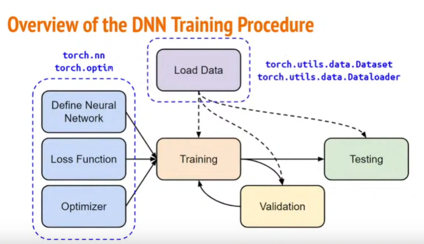
Objectives:
Solve a regression problem with deep neural networks (DNN).
Understand basic DNN training tips.
Get familiar with PyTorch.
If any questions, please contact the TAs via TA hours, NTU COOL, or email.
This code is completely written by Heng-Jui Chang @ NTUEE.
Copying or reusing this code is required to specify the original author.
E.g.
Source: Heng-Jui Chang @ NTUEE (https://github.com/ga642381/ML2021-Spring/blob/main/HW01/HW01.ipynb)
实验结构
实验环境
Google colab + GPU加速 + PyTorch
实验步骤
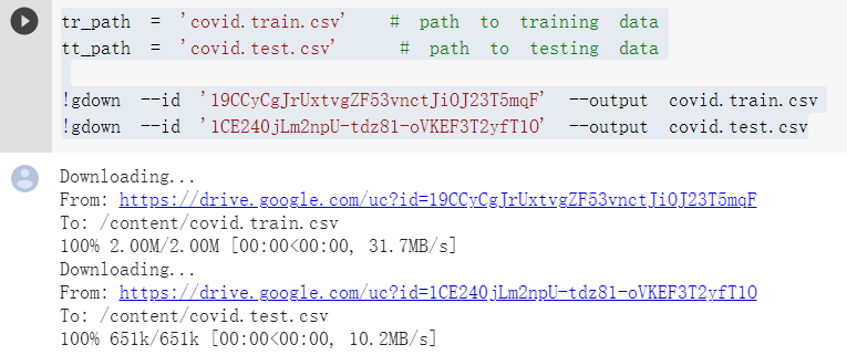
下载数据
tr_path = 'covid.train.csv'  # path to training data
tt_path = 'covid.test.csv'   # path to testing data
!gdown --id '19CCyCgJrUxtvgZF53vnctJiOJ23T5mqF' --output covid.train.csv
!gdown --id '1CE240jLm2npU-tdz81-oVKEF3T2yfT1O' --output covid.test.csv
output:
完成import以及确保可复现工作
# PyTorch
import torch
import torch.nn as nn
from torch.utils.data import Dataset, DataLoader

# For data preprocess
import numpy as np
import csv
import os

# For plotting
import matplotlib.pyplot as plt
from matplotlib.pyplot import figure

myseed = 42069  # set a random seed for reproducibility
torch.backends.cudnn.deterministic = True
torch.backends.cudnn.benchmark = False
np.random.seed(myseed)
torch.manual_seed(myseed)
if torch.cuda.is_available():
    torch.cuda.manual_seed_all(myseed)
最后一段单独拿出来解释(可以直接移步官方文档https://pytorch.org/docs/stable/notes/randomness.html)
REPRODUCIBILITY(复现性)
Completely reproducible results are not guaranteed across PyTorch releases, individual commits, or different platforms. Furthermore, results may not be reproducible between CPU and GPU executions, even when using identical seeds.

不保证跨 PyTorch 版本、单个提交或不同平台的完全可重现的结果。此外,即使使用相同的种子,结果也可能无法在 CPU 和 GPU 执行之间重现。

However, there are some steps you can take to limit the number of sources of nondeterministic behavior for a specific platform, device, and PyTorch release. First, you can control sources of randomness that can cause multiple executions of your application to behave differently. Second, you can configure PyTorch to avoid using nondeterministic algorithms for some operations, so that multiple calls to those operations, given the same inputs, will produce the same result.

但是,您可以采取一些步骤来限制特定平台、设备和 PyTorch 版本的非确定性行为来源的数量。首先,您可以控制可能导致应用程序多次执行以不同方式运行的随机源。其次,您可以配置 PyTorch 以避免对某些操作使用非确定性算法,以便在给定相同输入的情况下对这些操作的多次调用将产生相同的结果。
您可以使用torch.manual_seed()为所有设备(CPU 和 CUDA)设置 RNG:
import torch
torch.manual_seed(0)
if torch.cuda.is_available():
    torch.cuda.manual_seed_all(myseed)
对于自定义运算符,您可能还需要设置 python 种子:
import random
random.seed(0)
如果您或您使用的任何库依赖于 NumPy,您可以使用以下命令为全局 NumPy RNG 设置种子:
import numpy as np
np.random.seed(0)
CUDA 卷积操作使用的 cuDNN 库可能是应用程序多次执行的不确定性来源。当使用一组新的大小参数调用 cuDNN 卷积时,一个可选特征可以运行多个卷积算法,对它们进行基准测试以找到最快的算法。然后,最快的算法将在剩余的过程中一致地用于相应的大小参数集。由于基准测试噪声和不同的硬件,基准测试可能会在后续运行中选择不同的算法,即使是在同一台机器上。
禁用基准测试功能 会导致 cuDNN 确定性地选择算法,可能会以降低性能为代价。
torch.backends.cudnn.benchmark = False
但是,如果您不需要跨应用程序的多次执行的可重复性,那么可以使用 .
torch.backends.cudnn.benchmark = True
请注意,此设置与torch.backends.cudnn.deterministic 下面讨论的设置不同。
torch.use_deterministic_algorithms() 允许您将 PyTorch 配置为使用确定性算法而不是可用的不确定性算法,并在已知操作为不确定性(并且没有确定性替代方案)时抛出错误。
While disabling CUDA convolution benchmarking (discussed above) ensures that CUDA selects the same algorithm each time an application is run, that algorithm itself may be nondeterministic, unless either torch.use_deterministic_algorithms(True) or torch.backends.cudnn.deterministic = True is set. The latter setting controls only this behavior, unlike torch.use_deterministic_algorithms() which will make other PyTorch operations behave deterministically, too.
定义输出图象函数以及获取设备函数
def get_device():
''' Get device (if GPU is available, use GPU) '''
return 'cuda' if torch.cuda.is_available() else 'cpu'
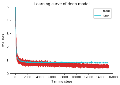
def plot_learning_curve(loss_record, title=''):
''' Plot learning curve of your DNN (train & dev loss) '''
total_steps = len(loss_record['train'])
x_1 = range(total_steps)
x_2 = x_1[::len(loss_record['train']) // len(loss_record['dev'])]
figure(figsize=(6, 4))
plt.plot(x_1, loss_record['train'], c='tab:red', label='train')
plt.plot(x_2, loss_record['dev'], c='tab:cyan', label='dev')
plt.ylim(0.0, 5.)
plt.xlabel('Training steps')
plt.ylabel('MSE loss')
plt.title('Learning curve of {}'.format(title))
plt.legend()
plt.show()
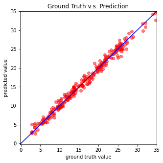
def plot_pred(dv_set, model, device, lim=35., preds=None, targets=None):
''' Plot prediction of your DNN '''
if preds is None or targets is None:
model.eval()
preds, targets = [], []
for x, y in dv_set:
x, y = x.to(device), y.to(device)
with torch.no_grad():
pred = model(x)
preds.append(pred.detach().cpu())
targets.append(y.detach().cpu())
preds = torch.cat(preds, dim=0).numpy()
targets = torch.cat(targets, dim=0).numpy()
figure(figsize=(5, 5))
plt.scatter(targets, preds, c='r', alpha=0.5)
plt.plot([-0.2, lim], [-0.2, lim], c='b')
plt.xlim(-0.2, lim)
plt.ylim(-0.2, lim)
plt.xlabel('ground truth value')
plt.ylabel('predicted value')
plt.title('Ground Truth v.s. Prediction')
plt.show()
We have three kinds of datasets:
train: for training
dev: for validation
test: for testing (w/o target value)
数据集
The COVID19Dataset below does:
- read
.csvfiles - extract features
- split
covid.train.csvinto train/dev sets - normalize features
Finishing TODO below might make you pass medium baseline.
class COVID19Dataset(Dataset):
    ''' Dataset for loading and preprocessing the COVID19 dataset '''
    def __init__(self,
                 path,
                 mode='train',
                 target_only=False):
        self.mode = mode

        # Read data into numpy arrays
        with open(path, 'r') as fp:
            data = list(csv.reader(fp))
            data = np.array(data[1:])[:, 1:].astype(float)

        if not target_only:
            feats = list(range(93))
        else:
            # TODO: Using 40 states & 2 tested_positive features (indices = 57 & 75)
            pass

        if mode == 'test':
            # Testing data
            # data: 893 x 93 (40 states + day 1 (18) + day 2 (18) + day 3 (17))
            data = data[:, feats]
            self.data = torch.FloatTensor(data)
        else:
            # Training data (train/dev sets)
            # data: 2700 x 94 (40 states + day 1 (18) + day 2 (18) + day 3 (18))
            target = data[:, -1]
            data = data[:, feats]

            # Splitting training data into train & dev sets
            if mode == 'train':
                indices = [i for i in range(len(data)) if i % 10 != 0]
            elif mode == 'dev':
                indices = [i for i in range(len(data)) if i % 10 == 0]

            # Convert data into PyTorch tensors
            self.data = torch.FloatTensor(data[indices])
            self.target = torch.FloatTensor(target[indices])

        # Normalize features (you may remove this part to see what will happen)
        self.data[:, 40:] = \
            (self.data[:, 40:] - self.data[:, 40:].mean(dim=0, keepdim=True)) \
            / self.data[:, 40:].std(dim=0, keepdim=True)

        self.dim = self.data.shape[1]

        print('Finished reading the {} set of COVID19 Dataset ({} samples found, each dim = {})'
              .format(mode, len(self.data), self.dim))

    def __getitem__(self, index):
        # Returns one sample at a time
        if self.mode in ['train', 'dev']:
            # For training
            return self.data[index], self.target[index]
        else:
            # For testing (no target)
            return self.data[index]

    def __len__(self):
        # Returns the size of the dataset
        return len(self.data)
必须提供方法 __getitem__ __len__以及 __init__ 作为接口向DataLoader提供服务。
加载数据
A DataLoader loads data from a given Dataset into batches.
def prep_dataloader(path, mode, batch_size, n_jobs=0, target_only=False):
    ''' Generates a dataset, then is put into a dataloader. '''
    dataset = COVID19Dataset(path, mode=mode, target_only=target_only)  # Construct dataset
    dataloader = DataLoader(
        dataset, batch_size,
        shuffle=(mode == 'train'), drop_last=False,
        num_workers=n_jobs, pin_memory=True)                            # Construct dataloader
    return dataloader
Deep Neural Network
NeuralNet is an nn.Module designed for regression. The DNN consists of 2 fully-connected layers with ReLU activation. This module also included a function cal_loss for calculating loss.
class NeuralNet(nn.Module):
    ''' A simple fully-connected deep neural network '''
    def __init__(self, input_dim):
        super(NeuralNet, self).__init__()

        # Define your neural network here
        # TODO: How to modify this model to achieve better performance?
        self.net = nn.Sequential(
            nn.Linear(input_dim, 64),
            nn.ReLU(),
            nn.Linear(64, 1)
        )

        # Mean squared error loss
        self.criterion = nn.MSELoss(reduction='mean')

    def forward(self, x):
        ''' Given input of size (batch_size x input_dim), compute output of the network '''
        return self.net(x).squeeze(1)

    def cal_loss(self, pred, target):
        ''' Calculate loss '''
        # TODO: you may implement L1/L2 regularization here
        return self.criterion(pred, target)
Training
def train(tr_set, dv_set, model, config, device):
    ''' DNN training '''

    n_epochs = config['n_epochs']  # Maximum number of epochs

    # Setup optimizer
    optimizer = getattr(torch.optim, config['optimizer'])(
        model.parameters(), **config['optim_hparas'])

    min_mse = 1000.
    loss_record = {'train': [], 'dev': []}      # for recording training loss
    early_stop_cnt = 0
    epoch = 0
    while epoch < n_epochs:
        model.train()                           # set model to training mode
        for x, y in tr_set:                     # iterate through the dataloader
            optimizer.zero_grad()               # set gradient to zero
            x, y = x.to(device), y.to(device)   # move data to device (cpu/cuda)
            pred = model(x)                     # forward pass (compute output)
            mse_loss = model.cal_loss(pred, y)  # compute loss
            mse_loss.backward()                 # compute gradient (backpropagation)
            optimizer.step()                    # update model with optimizer
            loss_record['train'].append(mse_loss.detach().cpu().item())

        # After each epoch, test your model on the validation (development) set.
        dev_mse = dev(dv_set, model, device)
        if dev_mse < min_mse:
            # Save model if your model improved
            min_mse = dev_mse
            print('Saving model (epoch = {:4d}, loss = {:.4f})'
                .format(epoch + 1, min_mse))
            torch.save(model.state_dict(), config['save_path'])  # Save model to specified path
            early_stop_cnt = 0
        else:
            early_stop_cnt += 1

        epoch += 1
        loss_record['dev'].append(dev_mse)
        if early_stop_cnt > config['early_stop']:
            # Stop training if your model stops improving for "config['early_stop']" epochs.
            break

    print('Finished training after {} epochs'.format(epoch))
    return min_mse, loss_record
Validation
def dev(dv_set, model, device):
    model.eval()                                # set model to evalutation mode
    total_loss = 0
    for x, y in dv_set:                         # iterate through the dataloader
        x, y = x.to(device), y.to(device)       # move data to device (cpu/cuda)
        with torch.no_grad():                   # disable gradient calculation
            pred = model(x)                     # forward pass (compute output)
            mse_loss = model.cal_loss(pred, y)  # compute loss
        total_loss += mse_loss.detach().cpu().item() * len(x)  # accumulate loss
    total_loss = total_loss / len(dv_set.dataset)              # compute averaged loss

    return total_loss
Testing
def test(tt_set, model, device):
    model.eval()                                # set model to evalutation mode
    preds = []
    for x in tt_set:                            # iterate through the dataloader
        x = x.to(device)                        # move data to device (cpu/cuda)
        with torch.no_grad():                   # disable gradient calculation
            pred = model(x)                     # forward pass (compute output)
            preds.append(pred.detach().cpu())   # collect prediction
    preds = torch.cat(preds, dim=0).numpy()     # concatenate all predictions and convert to a numpy array
    return preds
Setup Hyper-parameters
config contains hyper-parameters for training and the path to save your model.
device = get_device()                 # get the current available device ('cpu' or 'cuda')
os.makedirs('models', exist_ok=True)  # The trained model will be saved to ./models/
target_only = False                   # TODO: Using 40 states & 2 tested_positive features

# TODO: How to tune these hyper-parameters to improve your model's performance?
config = {
    'n_epochs': 3000,                # maximum number of epochs
    'batch_size': 270,               # mini-batch size for dataloader
    'optimizer': 'SGD',              # optimization algorithm (optimizer in torch.optim)
    'optim_hparas': {                # hyper-parameters for the optimizer (depends on which optimizer you are using)
        'lr': 0.001,                 # learning rate of SGD
        'momentum': 0.9              # momentum for SGD
    },
    'early_stop': 200,               # early stopping epochs (the number epochs since your model's last improvement)
    'save_path': 'models/model.pth'  # your model will be saved here
}
Load data and model
tr_set = prep_dataloader(tr_path, 'train', config['batch_size'], target_only=target_only)
dv_set = prep_dataloader(tr_path, 'dev', config['batch_size'], target_only=target_only)
tt_set = prep_dataloader(tt_path, 'test', config['batch_size'], target_only=target_only)

model = NeuralNet(tr_set.dataset.dim).to(device)  # Construct model and move to device
Start Training
model_loss, model_loss_record = train(tr_set, dv_set, model, config, device)
output
Saving model (epoch =    1, loss = 74.9742)
Saving model (epoch =    2, loss = 50.5313)
Saving model (epoch =    3, loss = 29.1148)
Saving model (epoch =    4, loss = 15.8134)
Saving model (epoch =    5, loss = 9.5430)
Saving model (epoch =    6, loss = 6.8086)
Saving model (epoch =    7, loss = 5.3892)
Saving model (epoch =    8, loss = 4.5267)
Saving model (epoch =    9, loss = 3.9454)
Saving model (epoch =   10, loss = 3.5560)
Saving model (epoch =   11, loss = 3.2303)
Saving model (epoch =   12, loss = 2.9920)
Saving model (epoch =   13, loss = 2.7737)
Saving model (epoch =   14, loss = 2.6181)
Saving model (epoch =   15, loss = 2.3987)
Saving model (epoch =   16, loss = 2.2712)
Saving model (epoch =   17, loss = 2.1349)
Saving model (epoch =   18, loss = 2.0210)
Saving model (epoch =   19, loss = 1.8848)
Saving model (epoch =   20, loss = 1.7999)
Saving model (epoch =   21, loss = 1.7510)
Saving model (epoch =   22, loss = 1.6787)
Saving model (epoch =   23, loss = 1.6450)
Saving model (epoch =   24, loss = 1.6030)
Saving model (epoch =   26, loss = 1.5052)
Saving model (epoch =   27, loss = 1.4486)
Saving model (epoch =   28, loss = 1.4069)
Saving model (epoch =   29, loss = 1.3733)
Saving model (epoch =   30, loss = 1.3533)
Saving model (epoch =   31, loss = 1.3335)
Saving model (epoch =   32, loss = 1.3011)
Saving model (epoch =   33, loss = 1.2711)
Saving model (epoch =   35, loss = 1.2331)
Saving model (epoch =   36, loss = 1.2235)
Saving model (epoch =   38, loss = 1.2180)
Saving model (epoch =   39, loss = 1.2018)
Saving model (epoch =   40, loss = 1.1651)
Saving model (epoch =   42, loss = 1.1631)
Saving model (epoch =   43, loss = 1.1394)
Saving model (epoch =   46, loss = 1.1129)
Saving model (epoch =   47, loss = 1.1107)
Saving model (epoch =   49, loss = 1.1091)
Saving model (epoch =   50, loss = 1.0838)
Saving model (epoch =   52, loss = 1.0692)
Saving model (epoch =   53, loss = 1.0681)
Saving model (epoch =   55, loss = 1.0537)
Saving model (epoch =   60, loss = 1.0457)
Saving model (epoch =   61, loss = 1.0366)
Saving model (epoch =   63, loss = 1.0359)
Saving model (epoch =   64, loss = 1.0111)
Saving model (epoch =   69, loss = 1.0072)
Saving model (epoch =   72, loss = 0.9760)
Saving model (epoch =   76, loss = 0.9672)
Saving model (epoch =   79, loss = 0.9584)
Saving model (epoch =   80, loss = 0.9526)
Saving model (epoch =   82, loss = 0.9494)
Saving model (epoch =   83, loss = 0.9426)
Saving model (epoch =   88, loss = 0.9398)
Saving model (epoch =   89, loss = 0.9223)
Saving model (epoch =   95, loss = 0.9111)
Saving model (epoch =   98, loss = 0.9034)
Saving model (epoch =  101, loss = 0.9014)
Saving model (epoch =  105, loss = 0.9011)
Saving model (epoch =  106, loss = 0.8933)
Saving model (epoch =  110, loss = 0.8893)
Saving model (epoch =  117, loss = 0.8867)
Saving model (epoch =  118, loss = 0.8867)
Saving model (epoch =  121, loss = 0.8790)
Saving model (epoch =  126, loss = 0.8642)
Saving model (epoch =  130, loss = 0.8627)
Saving model (epoch =  137, loss = 0.8616)
Saving model (epoch =  139, loss = 0.8534)
Saving model (epoch =  147, loss = 0.8467)
Saving model (epoch =  154, loss = 0.8463)
Saving model (epoch =  155, loss = 0.8408)
Saving model (epoch =  167, loss = 0.8354)
Saving model (epoch =  176, loss = 0.8314)
Saving model (epoch =  191, loss = 0.8267)
Saving model (epoch =  200, loss = 0.8212)
Saving model (epoch =  226, loss = 0.8190)
Saving model (epoch =  230, loss = 0.8144)
Saving model (epoch =  244, loss = 0.8136)
Saving model (epoch =  258, loss = 0.8095)
Saving model (epoch =  269, loss = 0.8076)
Saving model (epoch =  285, loss = 0.8064)
Saving model (epoch =  330, loss = 0.8055)
Saving model (epoch =  347, loss = 0.8053)
Saving model (epoch =  359, loss = 0.7992)
Saving model (epoch =  410, loss = 0.7989)
Saving model (epoch =  442, loss = 0.7966)
Saving model (epoch =  447, loss = 0.7966)
Saving model (epoch =  576, loss = 0.7958)
Saving model (epoch =  596, loss = 0.7929)
Saving model (epoch =  600, loss = 0.7893)
Saving model (epoch =  683, loss = 0.7825)
Saving model (epoch =  878, loss = 0.7817)
Saving model (epoch =  904, loss = 0.7794)
Saving model (epoch =  931, loss = 0.7790)
Saving model (epoch =  951, loss = 0.7781)
Saving model (epoch =  965, loss = 0.7771)
Saving model (epoch = 1018, loss = 0.7717)
Saving model (epoch = 1168, loss = 0.7653)
Saving model (epoch = 1267, loss = 0.7645)
Saving model (epoch = 1428, loss = 0.7644)
Saving model (epoch = 1461, loss = 0.7635)
Saving model (epoch = 1484, loss = 0.7629)
Saving model (epoch = 1493, loss = 0.7590)
Finished training after 1694 epochs
plot_learning_curve(model_loss_record, title='deep model')
output
del model
model = NeuralNet(tr_set.dataset.dim).to(device)
ckpt = torch.load(config['save_path'], map_location='cpu')  # Load your best model
model.load_state_dict(ckpt)
plot_pred(dv_set, model, device)  # Show prediction on the validation set
output
Testing
The predictions of your model on testing set will be stored at pred.csv.
def save_pred(preds, file):
    ''' Save predictions to specified file '''
    print('Saving results to {}'.format(file))
    with open(file, 'w') as fp:
        writer = csv.writer(fp)
        writer.writerow(['id', 'tested_positive'])
        for i, p in enumerate(preds):
            writer.writerow([i, p])

preds = test(tt_set, model, device)  # predict COVID-19 cases with your model
save_pred(preds, 'pred.csv')         # save prediction file to pred.csv
注:此次代码为助教提供,仅做部分解析,仅能通过base-line,后面blog提出改进

 浙公网安备 33010602011771号