《SEMI-SUPERVISED CLASSIFICATION WITH GRAPH CONVOLUTIONAL NETWORKS》论文阅读（二）

GCN的定义

下面内容参考kipf博客，个人认为是告诉你从直觉上，我们怎么得到GCN图上的定义（而前面的大幅推导是从理论上一步一步来的，也就是说可以用来佐证我们的直觉）

我们的网络输入是\(\mathcal{G}=(\mathcal{V},\mathcal{E})\)：

即可以用\(N\times D\)的矩阵\(X\)表示，\(N\)为图上结点个数，\(D\)是每个结点的特征维数
同时表示一个图还需要邻接矩阵\(A\)

而一层的输出记作\(Z_{\mathbb{R}^{N \times F}}\)，其中\(N\)还是结点个数，\(F\)为每个结点的特征维数

那么非线性神经网络就可以定义成如下形式：

\[H^{l+1}=f(H^{l}, A) \]

其中\(H^{0}=X\), \(H^{L}=Z\), \(L\) 表示网络的层数，那么模型的关键是如何设计\(f(\cdot )\)

一种简单的形式

\[f(H^{l}, A) = \sigma (AH^{l}W^{l}) \]

其中\(W^{l}\) 是\(l.th\)层的参数矩阵，\(\sigma ()\) 是激活函数。【PS:Despite its simplicity this model is already quite powerful】
仔细观察上式就能发现几个缺陷：

其中\(A\)是邻接矩阵，对角线上为\(0\)，导致经过网络中的一层，没有加上自己本结点的信息，所以改造替换成 \(\hat{A} = A+I\)
可是\(\hat {A}H\) 则是自己+相邻结点特征总和，还需平均化，所以改成 \(D^{-1}\hat {A}H\)
我们还可以更进一步，考虑到上篇说的拉普拉斯算子计算中周围结点总和\(-\)中心点*相邻结点个数，即相当于每个相邻点能量\(-\)中心点能量。类比过来，相邻点给我影响是:(相邻点能量/相邻点本身邻居个数)，所以有\(D^{-1/2}\hat{A}D^{-1/2}\)

\[f(H^{(l+1)}, A) = \sigma\left( D^{-\frac{1}{2}}\hat{A}D^{-\frac{1}{2}}H^{(l)}W^{(l)}\right) \, \]

这个形式已经和上篇利用谱理论推导处理的结果很相近了

\[\boldsymbol{g}_{\boldsymbol{\theta^{\prime}}} * \boldsymbol{x} = \theta(\boldsymbol{I_n} + \boldsymbol{D}^{-1/2} \boldsymbol{W} \boldsymbol{D}^{-1/2}) \boldsymbol{x} \]

但和最终的结果还不一样，回顾论文给的 renormalization trick：

\[I_{N}+D^{-1/2}AD^{-1/2}=D^{-1/2}\hat{A}D^{-1/2}\rightarrow \tilde{D}^{-1/2}\hat{A}\tilde{D}^{-1/2}=(D+I_{N})^{-1/2}\hat{A}(D+I_{N})^{-1/2} \]

\[\hat{A}=A+I_{N} \]

\[\tilde{D}_{ii}= \sum_{}^{j}\hat{A}_{ij}=D+I_{N} \]

那么的确可以得到最终形式：

\[f(H^{(l+1)}, A) = \sigma\left(\tilde{D}^{-\frac{1}{2}}\hat{A}\tilde{D}^{-\frac{1}{2}}H^{(l)}W^{(l)}\right) \, \]

WEISFEILER-LEHMAN算法

作者试图使用Weifeiler-Lehman算法来解释GCN的表征能力。\(WL\)算法是用来判断两个graph是否同构（简单说是两图拓扑结构相同）的，WL算法

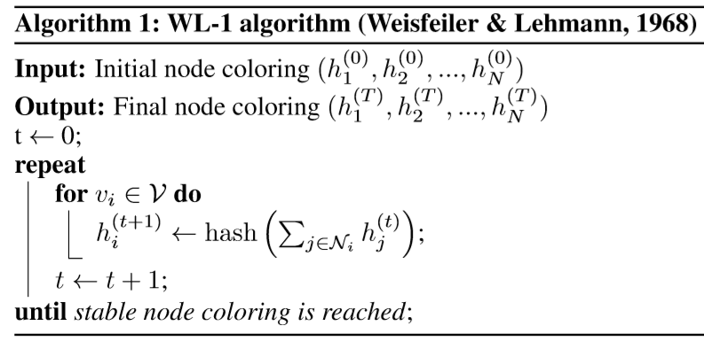
算法包含两个关键点

聚合自己和邻接结点信息，若记\(h\_aggregate^{t}_{i}\)，\(t\)是第几次迭代，\(i\) 是第几个结点
利用hash函数吐出唯一的值，\(h^{t+1}_{i}=hash(h\_aggregate^{t}_{i})\) 代替\(i\) 结点的特征

然后循环迭代

下面一个简单小例子（默认各个结点信息是相同的，所以序号均标为1，主要判断拓扑结构是否同构）：

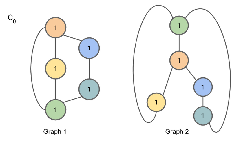
进行信息聚合，因为默认结点是一致的，所以主要通过邻接关系判断是否同构，\(\{1,1,1\}\)即是该结点的相邻结点是谁

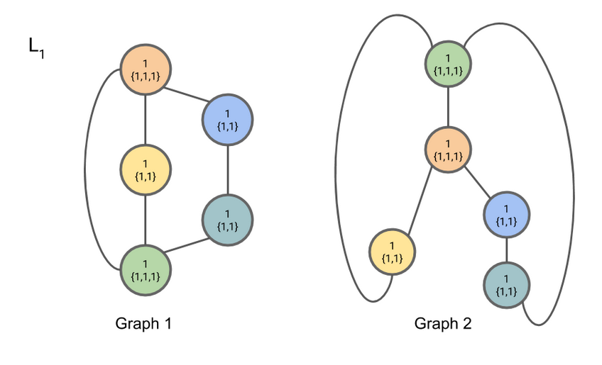
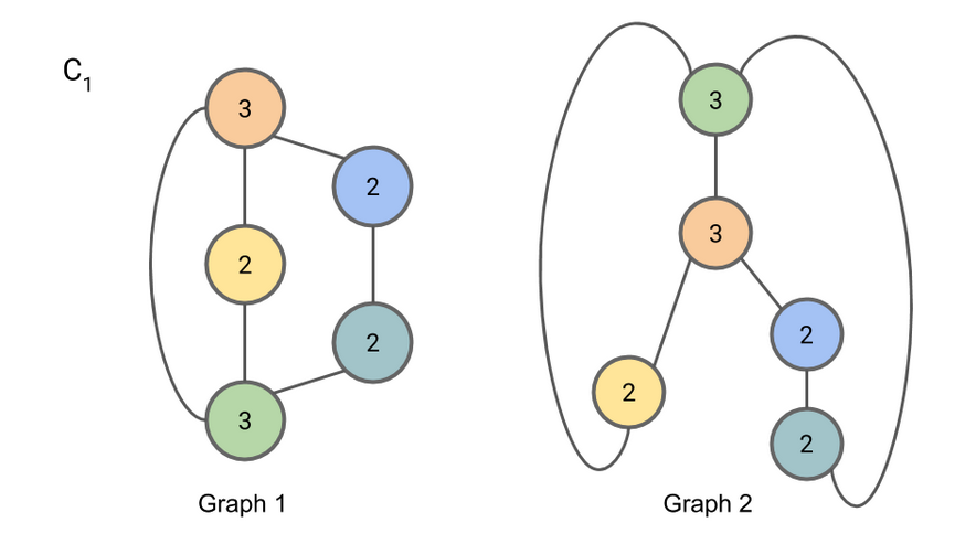
输入hash()函数，并且代替原有结点信息

重复上述操作（具体参见：https://www.davidbieber.com/post/2019-05-10-weisfeiler-lehman-isomorphism-test/#）
最后结果：

通过判断 \(9,8,7\) 两个图个数相同，判断是同构

WEISFEILER-LEHMAN算法反映什么

\(WL\)算法由于\(hash()\)函数的使用，使得通过不断迭代，能够表征不能不同结点的差异——即结点自身信息+结点的邻居所带来的差异

代替WL的hash()函数

\[h^{l+1}_{i}=\sigma (\sum_{j\in \mathcal{N_{i}}}^{}\frac{1}{c_{ij}}h_{j}^{l}W^{l}) \]

\(N_{i}\)是结点\(j\)的相邻结点，上式可进一步化成矩阵形式

\[h^{l+1}_{i}=\sigma (D^{-1/2}AD^{-1/2}h_{j}^{l}W^{l}) \]

通过调整\(W^{l}\)参数，实现\(hash()\)的功能。也就是说这种形式的GCN对结点的表征能力可以达到hash()函数级别，作者借此来证明GCN的能力。
可是有个疑问吧，这里用的是\(D^{-1/2}AD^{-1/2}\)，其实和上文提到的\(\tilde{D}^{-1/2}\hat{A}\tilde{D}^{-1/2}\)，也还是有区别的，前者不是GCN的最终形式。。。。

Zachary karate club举例

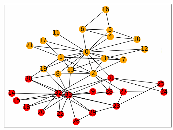
任务内容是酱紫的，一共有0~33位俱乐部成员，由于0号和33号两位之间发生了冲突，导致其他成员进行围绕这两位进行了“拉帮结派”，不同成员之间有一定交流（用连线表示），所以任务具体来说就是需要我们对这些成员进行分类——归属于哪个小团体。

我们先看一下label的真实分类情况：

import matplotlib.pyplot as plt
import networkx as nx
from networkx import karate_club_graph, to_numpy_matrix
import matplotlib.pyplot as plt

def lable_graph(G):

    fig,ax = plt.subplots()
    pos = nx.kamada_kawai_layout(G) # 指定图的美化排列方式

    cluter1 = []
    cluter2 = []
    for i in range(G.number_of_nodes()):
        if zkc.nodes[i]['club'] == 'Mr. Hi':
            cluter1.append(i)
        else:
            cluter2.append(i)
    nx.draw_networkx_nodes(G, pos, nodelist=cluter1,  node_color='orange')
    nx.draw_networkx_nodes(G, pos, nodelist=cluter2,  node_color='red')
    nx.draw_networkx_labels(G, pos, labels={i:str(i) for i in range(G.number_of_nodes())}, font_size=16)
    nx.draw_networkx_edges(G, pos, edgelist=G.edges())

zkc = karate_club_graph()
lable_graph(zkc)
plt.show()

假设暂时采用的形式进行研究：

\[D^{-1/2}\hat{A}D^{-1/2} \]

import numpy as np
import networkx as nx
import matplotlib.pyplot as plt
from networkx import karate_club_graph, to_numpy_matrix
# np.set_printoptions(threshold=np.inf)

zkc = karate_club_graph()
order = sorted(list(zkc.nodes()))
A = to_numpy_matrix(zkc, nodelist=order) # type=np.matrix

I = np.eye(A.shape[0])
A_hat = A + I

D_hat = np.diag(np.array(np.sum(A_hat, 0)).reshape(-1,))
# print(D_hat, D_hat.shape)
W1 = np.random.normal(loc=0, scale=1, size=(zkc.number_of_nodes(), 4))
W2 = np.random.normal(loc=0, scale=1, size=(W1.shape[1], 2))

def relu(x):
    return  1 / (1 + np.exp(-x))
    # return np.maximum(x, 0)

def gcn_layer(D_hat, A_hat, X, W):
    D_hat_1 = np.linalg.inv(D_hat)
    result = np.dot(D_hat_1, A).dot(X).dot(W)
    return relu(result)

H1 = gcn_layer(D_hat, A_hat, I, W1)
H2 = gcn_layer(D_hat, A_hat, H1, W2)
output = H2 # 34*2
# print(output, output.shape)

pos_weight = {
    node: (np.array(output)[node][0], np.array(output)[node][1])
    for node in zkc.nodes()}

def plot_graph_feature(G, pos_weight):
    fig, ax = plt.subplots()

    clsuter1 = []
    clsuter2 = []
    for i in range(G.number_of_nodes()):
        if G.nodes[i]['club'] == 'Mr. Hi':
            clsuter1.append(i)
        else:
            clsuter2.append(i)
    nx.draw_networkx_nodes(G, pos_weight, nodelist=clsuter1, node_color='orange')
    nx.draw_networkx_nodes(G, pos_weight, nodelist=clsuter2, node_color='red')
    nx.draw_networkx_labels(G, pos_weight, labels={i: str(i) for i in range(G.number_of_nodes())}, font_size=16)
    nx.draw_networkx_edges(G, pos_weight, edgelist=G.edges())


    ax.set_title('epoch')
    # x1_min = x1_max = pos_weight[0][0]
    # x2_min = x2_max = pos_weight[0][1]
    # for index,pos in pos_weight.items():
    #     x1_min = np.minimum(x1_min, pos[0])
    #     x1_max = np.maximum(x1_max, pos[0])
    #     x2_min = np.minimum(x2_min, pos[1])
    #     x2_max = np.maximum(x2_max, pos[1])
    # ax.set_xlim(x1_min, x1_max)
    # ax.set_ylim(x2_min, x2_max)

plot_graph_feature(zkc, pos_weight)
plt.show()

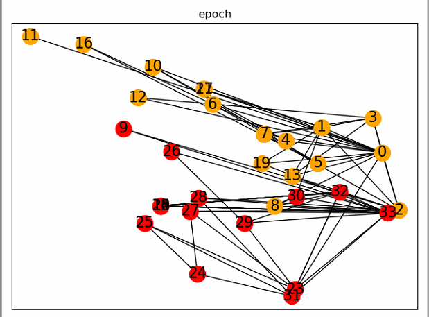
如上，采用随机初始化参数，配套使用两层GCN，根据\(WL\)理论，的确可以得到比较良好的分类结果（当然下图也是随机得到的比较理想的情况），但是我们都还没开始反向传播呢，效果有点闪瞎狗眼

使用DGL框架实现

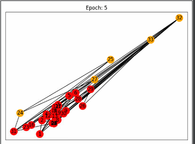
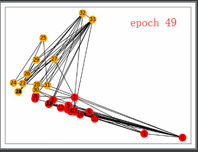
实现如下，总的来说，只使用了两个结点的label，最后的效果还是挺吃惊的，大有文章

import dgl
import numpy as np
import networkx as nx
import torch
import torch.nn as nn
import torch.nn.functional as F
from dgl.nn.pytorch import GraphConv
import itertools
import matplotlib.pyplot as plt


def build_karate_club_graph():
    src = np.array([1, 2, 2, 3, 3, 3, 4, 5, 6, 6, 6, 7, 7, 7, 7, 8, 8, 9, 10, 10,
                    10, 11, 12, 12, 13, 13, 13, 13, 16, 16, 17, 17, 19, 19, 21, 21,
                    25, 25, 27, 27, 27, 28, 29, 29, 30, 30, 31, 31, 31, 31, 32, 32,
                    32, 32, 32, 32, 32, 32, 32, 32, 32, 33, 33, 33, 33, 33, 33, 33,
                    33, 33, 33, 33, 33, 33, 33, 33, 33, 33])
    dst = np.array([0, 0, 1, 0, 1, 2, 0, 0, 0, 4, 5, 0, 1, 2, 3, 0, 2, 2, 0, 4,
                    5, 0, 0, 3, 0, 1, 2, 3, 5, 6, 0, 1, 0, 1, 0, 1, 23, 24, 2, 23,
                    24, 2, 23, 26, 1, 8, 0, 24, 25, 28, 2, 8, 14, 15, 18, 20, 22, 23,
                    29, 30, 31, 8, 9, 13, 14, 15, 18, 19, 20, 22, 23, 26, 27, 28, 29, 30,
                    31, 32])
    # Edges are directional in DGL; Make them bi-directional.
    u = np.concatenate([src, dst])
    v = np.concatenate([dst, src])
    # Construct a DGLGraph
    return dgl.DGLGraph((u, v))


def lable_gt_graph(G):
    fig, ax = plt.subplots()
    pos = nx.kamada_kawai_layout(G)  # 指定图的美化排列方式

    cluter1 = []
    cluter2 = []
    for i in range(G.number_of_nodes()):
        if G.nodes[i]['club'] == 'Mr. Hi':
            cluter1.append(i)
        else:
            cluter2.append(i)
    nx.draw_networkx_nodes(G, pos, nodelist=cluter1, node_color='orange')
    nx.draw_networkx_nodes(G, pos, nodelist=cluter2, node_color='red')
    nx.draw_networkx_labels(G, pos, labels={i: str(i) for i in range(G.number_of_nodes())}, font_size=16)
    nx.draw_networkx_edges(G, pos, edgelist=G.edges())


G = build_karate_club_graph()
# print('We have %d nodes.' % G.number_of_nodes())
# print('We have %d edges.' % G.number_of_edges())

nx_G = G.to_networkx().to_undirected()
# pos = nx.kamada_kawai_layout(nx_G)
# nx.draw(nx_G, pos, with_labels=True) # 未分类的
# plt.show()

embed = nn.Embedding(34, 5)  # 随机初始化
G.ndata['feat'] = embed.weight
# print(G.ndata['feat'][2])

class GCN(nn.Module):
    def __init__(self, in_feat, hidden_size, num_classes):
        super(GCN, self).__init__()
        self.conv1 = GraphConv(in_feat, hidden_size)
        self.conv2 = GraphConv(hidden_size, num_classes)

    def forward(self, g, inputs):
        h = self.conv1(g, inputs)
        h = torch.relu(h)
        h = self.conv2(g, h)
        return h


net = GCN(5, 5, 2)

inputs = embed.weight
labeled_nodes = torch.tensor([0, 33])
labels = torch.tensor([0, 1])

optimizer = torch.optim.Adam(itertools.chain(net.parameters(), embed.parameters()), lr=0.01)
all_logits = []

for epoch in range(50):
    logits = net(G, inputs)

    all_logits.append(logits.detach())

    logp = F.log_softmax(logits, 1)  # dimension

    loss = F.nll_loss(logp[labeled_nodes], labels)

    optimizer.zero_grad()
    loss.backward()
    optimizer.step()
   # print('Epoch %d | Loss: %.4f' % (epoch, loss.item()))

fig, ax = plt.subplots()
def draw(i):
    cls1color = 'orange'
    cls2color = 'red'
    pos = {}
    colors = []
    for v in range(34):
        pos[v] = all_logits[i][v].numpy()
        cls = pos[v].argmax()
        colors.append(cls1color if cls else cls2color)
    ax.set_title('Epoch: %d' % i)
    nx.draw_networkx(nx_G.to_undirected(), pos, node_color=colors,
                   node_size=300, with_labels=True)

    plt.show()

draw(5)
draw(49)