【计算几何】All in All

计算几何基础-初步

计算几何

定义：对几何外形信息的计算机表示分析。（其实就是利用计算机建立数学模型解决几何问题。）

计算几何研究的对象是几何图形。早期人们对于图像的研究一般都是先建立坐标系，把图形转换成函数，然后用插值和逼近的数学方法，特别是用样条函数作为工具来分析图形，取得了可喜的成功。然而，这些方法过多地依赖于坐标系的选取，缺乏几何不变性，特别是用来解决某些大挠度曲线及曲线的奇异点等问题时，有一定的局限性。

平面直角坐标系

平面直角坐标系其实就是笛卡尔坐标系，在计算几何中，我们经常会用到坐标表示，点和向量都是通过坐标来保存的。

向量及其运算

向量的基础知识

向量（也称为欧几里得向量、几何向量、矢量）：既有大小又有方向的量称为向量。在数学中研究的向量为自由向量，即只要不改变它的大小和方向，起点和终点可以任意平行移动的向量。记\(\vec{a}\)或a。

有向线段：带有方向的线段称为有向线段。有向线段三要素：起点，方向，长度，有了三要素，终点就唯一确定。我们用有向线段表示向量。

向量的模：有向线段\(\overrightarrow{AB}\)的长度称为向量的模，其实就是向量的大小。即为\(|\overrightarrow{AB}|\)或\(|\vec{a}|\)。

零向量：模为零的向量。零向量的方向任意。

单位向量：模为1的向量称为该方向上的单位向量。

平行向量：方向相同或相反的两个非零向量。记作\(a\parallel b\)。对于多个互相平行的向量，可以任作一条直线与这些向量平行，那么任一组平行向量都可以平移到同一直线上，所以平行向量又叫共线向量。

滑动向量：沿着直线作用的向量称为滑动向量。

固定向量：作用于一点的向量称为固定向量。

相等向量：模相等且方向相同的向量。

相反向量：模相等且方向相反的向量。

向量的夹角：已知两个非零向量\(\vec{a},\vec{b}\),作\(\overrightarrow{OA}=\vec{a},\overrightarrow{OB}=\vec{b}\)，那么$\theta=\angle AOB $ 就是向量\(\vec{a}\)与向量\(\vec{b}\)的夹角。记作：\(\left\langle a,b \right\rangle\)，显然当\(\theta=0\)时，两向量同向，\(\theta= \pi\)时两向量反向，\(\theta = \frac{\pi}{2}\)时，两向量垂直，记作\(\vec{a} \perp \vec{b}\)。并且我们规定\(\theta \in [0,\pi]\)。

\({\color{Red}注意}\)：平面向量具有方向性，我们并不能比较两个向量的大小（但可以比较两向量的模长）。但是两个向量可以相等。

向量的运算

设\(\vec{a}=(x_1,y_1)\),\(\vec{b}=(x_2,y_2)\)。

加减法

既然向量具有平移不变性，那么\(\vec{a}+\vec{b}\)就是将两条有向线段相连，即:\(\vec{a}+\vec{b}=(x_1+x_2,y_1+y_2)\)。

那向量的减法\(\vec{a}-\vec{b}\)，其实就是\(\vec{a}+(-\vec{b})\),即\(\vec{a}-\vec{b}=(x_1-x_2,y_1-y_2)\)。

向量的加减法是满足以下法则的：

• 三角形法则：若要求和的向量首尾顺次相连，那么这些向量的和为第一个向量的起点指向最后一个向量的终点；
• 平行四边形法则：若要求和的两个向量共起点，那么它们的和向量为以这两个向量为邻边的平行四边形的对角线，起点为两个向量共有的起点，方向沿平行四边形对角线方向。

所以说向量的加减法就有了几何意义，并且满足交换律和结合律。

数乘

规定\(\left\lceil 实数\lambda与向量\vec{a}的积 \right\rfloor\)为一个向量，这种运算就是数乘。记作\(\lambda\vec{a}\),并且满足以下性质：

• \(|\lambda\vec{a}|=|\lambda||\vec{a}|\)；
• 当\(\lambda>0\)时，\(\lambda\vec{a}\)与\(\vec{a}\)同向，当\(\lambda=0\)时，\(\lambda\vec{a}=0\)，当\(\lambda<0\)时，\(\lambda\vec{a}\)与\(\vec{a}\)方向相反。

\[\lambda(\mu\vec{a})=(\lambda\mu)\vec{a}\\ (\lambda+\mu)\vec{a}=\lambda\vec{a}+\mu\vec{a}\\ \lambda(\vec{a}+\vec{b})=\lambda\vec{a}+\lambda\vec{b}\\ (-\lambda)\vec{a}=-(\lambda\vec{a})=-\lambda(\vec{a})\\ \lambda(\vec{a}-\vec{b})=\lambda\vec{a}-\lambda\vec{b} \]

（向量的数乘其实就是对向量进行放缩）

点积

向量的点积也叫数量积、内积，向量的点积表示为\(\vec{a}·\vec{b}\),是一个实数。计算式为：

\[\vec{a}·\vec{b}=|\vec{a}||\vec{b}|cos\theta(\theta=\left\langle \vec{a},\vec{b} \right\rangle)(\theta表示\vec{a},\vec{b}的夹角) \]

三角形恒等变换的推导：

\[\because \vec{a}·\vec{b}=|\vec{a}||\vec{b}|cos\theta\\ \therefore \vec{a}·\vec{b}=\sqrt{(x_1)^2+(y_1)^2}·\sqrt{(x_2)^2+(y_2)^2}·cos\theta\\ \because cos\theta=cos(\alpha-\beta)=cos\alpha cos\beta + sin\alpha sin\beta\\ \because cos\alpha=\dfrac{x_1}{\sqrt{(x_1)^2+(y_1)^2}},sin\alpha=\dfrac{x_1}{\sqrt{(y_1)^2+(y_1)^2}}\\ cos\beta=\dfrac{x_2}{\sqrt{(x_2)^2+(y_2)^2}},sin\beta=\dfrac{y_2}{\sqrt{(x_2)^2+(y_2)^2}}\\ \therefore 整理代入得：\vec{a}·\vec{b}=x_1x_2+y_1y_2 \]

同时点积是满足交换律，结合律和分配律的。

点积应用：

叉积

也叫矢量积，外积。几何意义是两向量由平行四边形法则围成的面积。叉积是一个向量，垂直于原来两个向量所在的平面。（根据叉乘的模是平行四边形的面积我们可以想象，叉乘的结果是一个有方向的面，而面的方向平行于面的法线，所以面的方向垂直于面上任何一个向量），即：

\[|\vec{a} × \vec{b}|=|\vec{a}||\vec{b}|sin\left\langle a,b \right\rangle \]

并且，\(\vec{a}×\vec{b}=(x_1y_2-x_2y_2)\)。

叉积是一个有向面积：

• \(\vec{a}×\vec{b}=0\)，等价于\(\vec{a},\vec{b}\)，共线（可以反向）；
• \(\vec{a}×\vec{b}>0\)，\(\vec{b}\)在\(\vec{a}\)左侧；
• \(\vec{a}×\vec{b}<0\)，\(\vec{b}\)在\(\vec{a}\)右侧。

判断两向量共线

两个非零向量\(\vec{a}\)与\(\vec{b}\)共线\(\iff\)有唯一实数\(\lambda\)，使得\(\vec{b}=\lambda\vec{a}\)。由向量的数乘即可得证。

推论：如果\(l\)为已经过点A且平行于已知非零向量\(\vec{a}\)的直线，那么对空间任一点O，点P在直线\(l\)上的充要条件是存在实数\(t\)，满足等式：\(\vec{OP}=\vec{OA}+t\vec{a}\)。

其中向量\(\vec{a}\)叫做直线\(l\)的方向向量。

基本定理和坐标表示

平面向量基本定理

平面向量基本定理：两个向量\(\vec{a}\)和\(\vec{b}\)不共线的充要条件是，对于和向量\(\vec{a}\)，\(\vec{b}\)共面的任意向量\(\vec{p}\)，有唯一实数对\((x,y)\)满足\(\vec{p}=x\vec{a}+y\vec{b}\)。

证明(非常简单):

\[对于平面上的任意向量可以沿指定方向被分解为任意两个向量，\\ 平面上的任意两个向量可以沿指定方向合成任意指定向量。\\ 对于有唯一实数对我们可以用反证法:\\ 假设有两个及以上的实数对满足要求为(m,n)\\ \therefore x\vec{a}+y\vec{b}=m\vec{a}+n\vec{b}\\ \therefore (x-m)\vec{a}=(n-y)\vec{b}\\ \because \vec{a}和\vec{b}不共线\\ \therefore x=m,n=y\\ 与假设矛盾所以结论成立\\证毕 \]

在同一平面内的两个不共线的向量称为基底。

如果基底相互垂直，那么我们在分解的时候就是对向量正交分解。

平面向量的坐标表示

如果取与横轴与纵轴方向相同的单位向量\(i,j\)作为一组基底，根据平面向量基本定理，平面上的所有向量与有序实数对\((x,y)\)一一对应。

而有序实数对

而有序数对\((x,y)\)与平面直角坐标系上的点一一对应，那么我们作\(\vec{OP}=\vec{p}\)，那么终点\(P(x,y)\)也是唯一确定的。由于我们研究的都是自由向量，可以自由平移起点，这样，在平面直角坐标系里，每一个向量都可以用有序实数对唯一表示。

坐标运算

平面向量线性运算

由平面向量的线性运算，我们可以推导其坐标运算，主要方法是将坐标全部化为用基底表示，然后利用运算律进行合并，之后表示出运算结果的坐标形式。

对于向量\(\vec{a}=(m,n)\)和向量\(\vec{b}=(p,q)\)，则有：

\[\vec{a}+\vec{b}=(m+n,n+q)\\ \vec{a}-\vec{b}=(m-n,n-q)\\ k\vec{a}=(km,kn),k\vec{b}=(kq,kq) \]

向量的坐标表示

已知两点\(A(a,b),B(c,d)\),则\(\vec{AB}=(c-a,d-b)\)。

平移一点

将一点\(P\)沿一定方向平移某单位长度，只需要将要平移的方向和距离组合成一个向量，利用三角形法则，用\(\vec{OP}\)加上这个向量即可，得到的向量终点即为平移后的点。

三点共线的判定

在平面上\(A,B,C\)三点共线的充要条件是：\(\vec{OC}=\lambda\vec{OB}+(1-\lambda)\vec{OA},(O为平面内不与直线AC共线任意一点)\)。

证明：

\[若点B与AC共线，由共线向量定理可知：\vec{AC}=\lambda\vec{AB}\\ \therefore \vec{AC}=\lambda\vec{AB}\iff\vec{OC}-\vec{OA}=\lambda(\vec{OB}-\vec{OA})\iff\vec{OC}=(1-\lambda)\vec{OA}+\lambda\vec{OB}\\ 证毕 \]

计算几何-凸包

二维凸包

凸多边形

凸多边形是指所有内角在\(\left[ 0,\pi \right]\)范围内的简单多边形。

凸包

对于在平面上的一个点集，凸包是能包含所有点的最小凸多边形。

其定义为：对于给定集合\(D\)，所有包含\(D\)的凸集的交集\(S\)被称为\(D\)的凸包。

如：

凸包求法

对于平面上的一个点集，其凸包可以用分治，\(Graham-Scan\)，和 \(Andrew\)。

分治

对于分治算法解决凸包问题，递归求解，找到子问题的凸包，讲左右两个子集的凸包进进行合并即可，时间复杂度\((n \log n)\)。

\(Andrew\)

对于\(Andrew\)算法，主要流程：

• 首先将所有点以横坐标为第一关键字，纵坐标为第二关键字进行排序；

• 显然排序后最小的元素和最大的元素一定在凸包上，然后用单调栈维护上下凸壳；

• 因为上下凸壳所旋转的方向不同，我们首先升序枚举下凸壳，然后降序枚举上凸壳。

时间复杂度\((n \log n)\)。

\(Graham-Scan\)

主要介绍这种算法，更好写一些，首先我们先找出在最右下角的点，此时这个点一定在凸包上，然后我们从这个点开始逆时针旋转，同时用单调栈维护凸包上的点，每加入一个新点是判断改点是否会出现，该边在上一条边的“右边”，如果出现则删除上一个点。

【模板】二维凸包

Code:

#include<bits/stdc++.h>
using namespace std;
const int maxn=1e5+10;
int n,top;double ans;
struct geometric{
    double x,y,dss;
    friend geometric operator + (const geometric a,const geometric b){return (geometric){a.x+b.x,a.y+b.y};} 
    friend geometric operator - (const geometric a,const geometric b){return (geometric){a.x-b.x,a.y-b.y};} 
    double dis(geometric a,geometric b){return sqrt((a.x-b.x)*(a.x-b.x)+(a.y-b.y)*(a.y-b.y));}
    double dot(geometric a1,geometric a2,geometric b1,geometric b2){return (a2.x-a1.x)*(b2.x-b1.x)+(a2.y-a1.y)*(b2.y-b1.y);}
    double cross(geometric a1,geometric a2,geometric b1,geometric b2){return (a2.x-a1.x)*(b2.y-b1.y)-(a2.y-a1.y)*(b2.x-b1.x);}
};
geometric origin,data[maxn],st[maxn];
bool vis[maxn];
bool cmp(geometric a,geometric b)
{
    geometric opt;
    double tamp=opt.cross(data[1],a,data[1],b);
    if(tamp>0)return true;
    if(tamp==0&&opt.dis(data[1],a)<=opt.dis(data[1],b))return true;
    return false;
}
geometric opt;
int main()
{
    scanf("%d",&n);
    for(int i=1;i<=n;i++)
    {
        scanf("%lf%lf",&data[i].x,&data[i].y);
        if(i!=1&&data[i].y<data[1].y)
        {   
            double tmp;
            swap(data[1].y,data[i].y);
            swap(data[1].x,data[i].x);
        }
        if(i!=1&&data[i].y==data[1].y&&data[i].x>data[1].x)
        	swap(data[1].x,data[i].x);
    }
    sort(data+2,data+n+1,cmp);
    st[++top]=data[1];
    for(int i=2;i<=n;i++)
    {
        while(top>1&&opt.cross(st[top-1],st[top],st[top],data[i])<=0)top--;
        st[++top]=data[i];
    }
    st[++top]=data[1];
    for(int i=1;i<top;i++)ans+=opt.dis(st[i],st[i+1]);
    printf("%.2lf",ans);
    return 0;
}

动态凸包

首先我们考虑这样一个问题：

两种操作：

• 向点集中添加一个点\((x,y)\);
• 询问点是否在凸包中。

首先我们对于一个动态的凸包，很明显在每次加入新点时不能再进行一次\(Graham-Scan\)，否则时间复杂度不优。

那么我们就可以用一下方法：

• 首先建一棵平衡树，按极角排序；

• 询问是找到该点的前驱后继，用叉积判断即可，否则执行插入操作；

• 插入时，先将点插入平衡树内然后找该点的前驱后继，同时不断去旋转将在凸包内的点删去。

对于平衡树我们可以直接用\(STL\)里的\(set\) 去实现，需要用到迭代器。

Professor's task

Code:

#include<bits/stdc++.h>
#define it set<geometric>::iterator
#define eps 1e-8
using namespace std;
const int maxn=1e5+10;
int Sure(double x){return fabs(x)<eps?0:(x<0?-1:1);}
struct geometric{
    double x,y;
    geometric(double X=0,double Y=0):x(X),y(Y) {}
    friend geometric operator + (const geometric a,const geometric b){return geometric(a.x+b.x,a.y+b.y);} 
    friend geometric operator - (const geometric a,const geometric b){return geometric(a.x-b.x,a.y-b.y);} 
    friend geometric operator * (const geometric a,double p){return geometric(a.x*p,a.y*p);}
    friend geometric operator / (const geometric a,double p){return geometric(a.x/p,a.y/p);}
    double dis(geometric a,geometric b){return sqrt((a.x-b.x)*(a.x-b.x)+(a.y-b.y)*(a.y-b.y));}
    double dot(geometric a1,geometric a2,geometric b1,geometric b2){return (a2.x-a1.x)*(b2.x-b1.x)+(a2.y-a1.y)*(b2.y-b1.y);}
    double cross(geometric a1,geometric a2,geometric b1,geometric b2){return (a2.x-a1.x)*(b2.y-b1.y)-(a2.y-a1.y)*(b2.x-b1.x);}
    double corner(geometric a1,geometric a2,geometric b1,geometric b2){return dot(a1,a1,b1,b2)/(dis(a1,a2)*dis(b1,b2));}
    double area(geometric a1,geometric a2,geometric b1,geometric b2){return fabs(cross(a1,a2,b1,b2));}
    double angle(geometric a){return atan2(a.y,a.x);}
    geometric rotate_clockwise(geometric a,double theta){return geometric(a.x*cos(theta)-a.y*sin(theta),a.x*sin(theta)+a.y*cos(theta));}
    geometric rotate_counterclockwise(geometric a,double theta){return geometric(a.x*cos(theta)+a.y*sin(theta),-a.x*sin(theta)+a.y*cos(theta));}
}opt,d[maxn],origin;
bool operator < (geometric a,geometric b){
    a=a-origin;b=b-origin;
    double ang1=atan2(a.y,a.x),ang2=atan2(b.y,b.x);
    double l1=sqrt(a.x*a.x+a.y*a.y),l2=sqrt(b.x*b.x+b.y*b.y);
    if(Sure(ang1-ang2)!=0)return Sure(ang1-ang2)<0;
    else return Sure(l1-l2)<0;
}
int q,cnt;
set<geometric> S;
it Pre(it pos){if(pos==S.begin())pos=S.end();return --pos;}
it Nxt(it pos){++pos; return pos==S.end() ? S.begin():pos;}
bool Query(geometric key)
{
    it pos=S.lower_bound(key);
    if(pos==S.end())pos=S.begin();
    return Sure(opt.cross(*(Pre(pos)),key,*(Pre(pos)),*(pos)))<=0;
}
void Insert(geometric key)
{
    if(Query(key))return;
    S.insert(key);
    it pos=Nxt(S.find(key));
    while(S.size()>3&&Sure(opt.cross(*(Nxt(pos)),*(pos),*(Nxt(pos)),key))>=0)
    {
        S.erase(pos);pos=Nxt(S.find(key));
    }
    pos=Pre(S.find(key));
    while(S.size()>3&&Sure(opt.cross(*(Pre(pos)),*(pos),*(Pre(pos)),key))<=0)
    {
        S.erase(pos);pos=Pre(S.find(key));
    }
}
int main()
{
    scanf("%d",&q);
    for(int i=1;i<=3;i++)
    {
        int opt;double x,y;scanf("%d%lf%lf",&opt,&x,&y);
        d[++cnt]=geometric(x,y);origin.x+=x;origin.y+=y;
    }
    origin=origin/3.0;
    for(int i=1;i<=3;i++)S.insert(d[i]);
    for(int i=4;i<=q;i++)
    {
        int opt;double x,y;
        scanf("%d%lf%lf",&opt,&x,&y);
        d[++cnt]=geometric(x,y);
        if(opt==1)Insert(d[cnt]);
        else {
            if(Query(d[cnt]))printf("YES\n");
            else printf("NO\n");
        }
    }
    return 0;
}

注意使用迭代器时不要越界，要和用指针一样小心！

三维凸包

咕咕咕

对于$\vec{a} (x_1,y_1) $

和\(\vec{b}(x_2,y_2)\)

三维凸包的话，主要是空间几何坐标系中点积为：

\[ \vec{a} · \vec{b} = x_1x_2+y_1y_2+z_1z_2 \]

叉积为向量（法向量）：

\[ \vec{a} \times \vec{b} =(y_1z_2 - y_2z_1, x_2z_1-z_2x_1, x_1y_2 -x_2y_1) \]

【模板】三维凸包

Code:

#include<bits/stdc++.h>
#define eps 1e-10
#define double long double
using namespace std;
const int maxn=2010;
double randeps(){return (rand()/(double)RAND_MAX-0.5)*eps;}
struct geometric{
    double x,y,z;
    geometric(double X=0,double Y=0,double Z=0):x(X),y(Y),z(Z) {}
    void shake(){x+=randeps(),y+=randeps(),z+=randeps();}
    friend geometric operator + (const geometric a,const geometric b){return geometric(a.x+b.x,a.y+b.y,a.z+b.z);} 
    friend geometric operator - (const geometric a,const geometric b){return geometric(a.x-b.x,a.y-b.y,a.z-b.z);} 
    friend geometric operator * (const geometric a,double p){return geometric(a.x*p,a.y*p,a.z*p);}
    friend geometric operator / (const geometric a,double p){return geometric(a.x/p,a.y/p,a.z/p);}// 向量的四则运算
    double dis(geometric a,geometric b){return sqrt((a.x-b.x)*(a.x-b.x)+(a.y-b.y)*(a.y-b.y)+(a.z-b.z)*(a.z-b.z));} // 向量模长
    double dot(geometric a1,geometric a2,geometric b1,geometric b2){return (a2.x-a1.x)*(b2.x-b1.x)+(a2.y-a1.y)*(b2.y-b1.y)+(a2.z-a1.z)*(b2.z-b1.z);}// 点积
    geometric cross(geometric a1,geometric a2,geometric b1,geometric b2){geometric a=a2-a1,b=b2-b1;return geometric(a.y*b.z-b.y*a.z,b.x*a.z-a.x*b.z,a.x*b.y-b.x*a.y);} // 叉积
}opt,origin,p[maxn];
struct plane{
    int v[3];
    plane(){v[0]=v[1]=v[2]=0;}
    plane(int A,int B,int C){v[0]=A,v[1]=B,v[2]=C;}
    geometric normal(){return opt.cross(p[v[0]],p[v[1]],p[v[0]],p[v[2]]);}
    double area(){return fabs(opt.dis(normal(),origin))/2.0;}
}con[maxn<<1],h[maxn<<1];
int check(plane alpha,geometric vec){return opt.dot(origin,alpha.normal(),p[alpha.v[0]],vec)>0;}
int n,cnt,indx,l,vis[maxn][maxn];double S;
int main()
{
    srand(time(0));
    scanf("%d",&n);
    for(int i=1;i<=n;i++)
    {
        double x,y,z;
        scanf("%Lf%Lf%Lf",&x,&y,&z);
        p[++cnt]=geometric(x,y,z);
        p[i].shake();
    }
    con[++indx]=plane(1,2,3);
    con[++indx]=plane(3,2,1);
    for(int i=4;i<=cnt;i++)
    {
        for(int j=1,res;j<=indx;j++)
        {
            res=check(con[j],p[i]);
            if(!res)h[++l]=con[j];
            for(int k=0;k<3;k++)
            {
                vis[con[j].v[k]][con[j].v[(k+1)%3]]=res;
            }
        }
        for(int j=1;j<=indx;j++)
        {
            for(int k=0;k<3;k++)
            {
                int x=con[j].v[k],y=con[j].v[(k+1)%3];
                if(vis[x][y]&&!vis[y][x])h[++l]=plane(x,y,i);
            }
        }
        for(int j=1;j<=l;j++)con[j]=h[j];
        indx=l,l=0;
    }
    for(int i=1;i<=indx;i++)S+=con[i].area();
    printf("%0.3Lf",S);
    return 0;
}

一些例题：

[SHOI2012]信用卡凸包

[HAOI2011]防线修建

[HNOI2008]水平可见直线

[SDOI2013]保护出题人

计算几何-旋转卡壳

读法

（其实我也不知道该怎么读，有16种读法）

$ xu\grave{a}n $ $ zhu\grave{a}n $ $ qi\check{a} $ $ qi\grave{a}o $

$ \huge{旋转卡壳}$

凸多边形的切线

如果一条直线与凸多边形有交点，并且整个凸多边形都在这条直线的一侧，那么这条直线就是该凸多边形的一条切线。

对踵点

如果过凸多边形上两点作一对平行线，使得整个多边形都在这两条线之间，那么这两个点被称为一对对踵点。

凸多边形的直径

即凸多边形上任意两个点之间距离的最大值。直径一定会在对踵点中产生，如果两个点不是对踵点，那么两个点中一定可以让一个点向另一个点的对踵点方向移动使得距离更大。并且点与点之间的距离可以体现为线与线之间的距离，在非对踵点之间构造平行线，一定没有在对踵点构造平行线优，这一点可以通过平移看出。

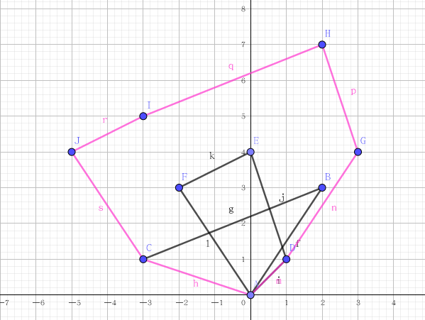
旋转卡壳

先上一张比较标致的图，来对旋转卡壳有一个初步的了解：

对于实现旋转卡壳，我们首先可以先去求出凸包，然后去枚举每一条边，去找对踵点，即可找出凸包直径。时间复杂度\(O(n \log n)\)

在旋转的时候用叉积对应的面积，来找对踵点就好了，因为在凸包上有一个单调性，在找对踵点的时候，实际上是\(O(n)\)的，建议好好思考一下。

\(\color{red} {注意，在旋转时为一个环，需要注意边界问题，要不要会收获血与泪的教训}\) （别问我怎么知道的）

【模板】旋转卡壳

Code:

#include<bits/stdc++.h>
using namespace std;
const int maxn=5e4+10;
struct geometric{
    double x,y,dss;
    friend geometric operator + (const geometric a,const geometric b){return (geometric){a.x+b.x,a.y+b.y};} 
    friend geometric operator - (const geometric a,const geometric b){return (geometric){a.x-b.x,a.y-b.y};} 
    double dis(geometric a,geometric b){return sqrt((a.x-b.x)*(a.x-b.x)+(a.y-b.y)*(a.y-b.y));}
    double dot(geometric a1,geometric a2,geometric b1,geometric b2){return (a2.x-a1.x)*(b2.x-b1.x)+(a2.y-a1.y)*(b2.y-b1.y);}
    double cross(geometric a1,geometric a2,geometric b1,geometric b2){return (a2.x-a1.x)*(b2.y-b1.y)-(a2.y-a1.y)*(b2.x-b1.x);}
    double corner(geometric a1,geometric a2,geometric b1,geometric b2){return dot(a1,a1,b1,b2)/(dis(a1,a2)*dis(b1,b2));}
};
int n,top;double ans;
geometric d[maxn],opt,st[maxn];
bool cmp(geometric a,geometric b)
{
    double tamp=opt.cross(d[1],a,d[1],b);
    if(tamp>0)return true;
    if(tamp==0&&opt.dis(d[1],a)<opt.dis(d[1],b))return true;
    return false;
}
int main()
{
    scanf("%d",&n);
    for(int i=1;i<=n;i++)
    {
        scanf("%lf%lf",&d[i].x,&d[i].y);
        if(i!=1&&d[i].y<d[1].y)
        {
            swap(d[1].y,d[i].y);
            swap(d[1].x,d[i].x);
        }
        if(i!=1&&d[i].y==d[1].y&&d[i].x>d[1].x)
            swap(d[1].x,d[i].x);
    }
    sort(d+2,d+n+1,cmp);
    st[++top]=d[1];
    for(int i=2;i<=n;i++)
    {
        while(top>1&&opt.cross(st[top-1],st[top],st[top],d[i])<=0)top--;
        st[++top]=d[i];
    }
    st[++top]=d[1];
    for(int i=2,j=3;i<=top;i++)
    {
        while(opt.cross(st[i-1],st[i],st[i-1],st[j])<opt.cross(st[i-1],st[i],st[i-1],st[j+1]))j==top-1?j=1:j++;// ！！！！
        ans=max(ans,max(opt.dis(st[i],st[j]),opt.dis(st[i-1],st[j])));
    }
    printf("%d",int(ans*ans));
    return 0;
}

一些例题

[HNOI2007]最小矩形覆盖

[SCOI2007]最大土地面积

[HNOI2008]水平可见直线

[ZJOI2008]瞭望塔

部分资料参考自洛谷日报

计算几何-半平面交

半平面

平面内的一条直线把这个平面分成两部分，每一部分对这个平面来说，都叫做半平面。包括这条直线的半平面叫做闭半平面，否则叫做开半平面。

解析式为 \(Ax + By +C >=0\)或\(Ax + By +C <=0\)。

在计算几何中用向量表示，整个题统一以向量的左侧或右侧为半平面。

半平面交

半平面交就是多个半平面的交集。半平面交是一个点集。

它可以理解为向量集中每一个向量的右侧的交，或者是下面方程组的解。

\[ \begin{equation} \begin{cases} A1x+B1y+C1\ge0\newline A2x+B2y+C2\ge0\newline ~~~~~~~~~~~~~~\dots \end{cases} \end{equation} \]

多边形的核

如果一个点集中的点与多边形上任意一点的连线与多边形没有其他交点，那么这个点集被称为多边形的核。

把多边形的每条边看成是首尾相连的向量，那么这些向量在多边形内部方向的半平面交就是多边形的核。

求法

D&C算法

该算法是基于分治思想的：

• 将\(n\)个半平面分成两个\(n/2\)的集合;

• 对两个子集和递归求解半平面交;

• 将前一步算出来的两个交利用平面扫描法求解。

时间复杂度\((n \log n)\)这个算法并不常用，主要介绍的是下面这个。

S&I算法

该算法是在2006年有中国队队员朱泽园提出来的“排序增量法”。

假设给出\(n\)条直线，求这\(n\)条直线的左方半平面的交集：

• 首先对这\(n\)条直线按极角排序；

• 用一个队列去维护半平面的交集，和相邻两条直线的交点；

• 每次加入新的直线时判断是否有交点在该直线的右面，如果是则弹出直线，先判队尾再判队首，注意判断平行情况；

• 最后队列中的交集即为半平面交。

【模板】半平面交

Code:

#include<bits/stdc++.h>
#define eps 1e-8
using namespace std;
const int maxn=1010;
struct geometric{
    double x,y;
    geometric(double X=0,double Y=0):x(X),y(Y) {}
    friend geometric operator + (const geometric a,const geometric b){return geometric(a.x+b.x,a.y+b.y);} 
    friend geometric operator - (const geometric a,const geometric b){return geometric(a.x-b.x,a.y-b.y);} 
    friend geometric operator * (const geometric a,double p){return geometric(a.x*p,a.y*p);}
    friend geometric operator / (const geometric a,double p){return geometric(a.x/p,a.y/p);}
    double dis(geometric a,geometric b){return sqrt((a.x-b.x)*(a.x-b.x)+(a.y-b.y)*(a.y-b.y));}
    double dot(geometric a1,geometric a2,geometric b1,geometric b2){return (a2.x-a1.x)*(b2.x-b1.x)+(a2.y-a1.y)*(b2.y-b1.y);}
    double cross(geometric a1,geometric a2,geometric b1,geometric b2){return (a2.x-a1.x)*(b2.y-b1.y)-(a2.y-a1.y)*(b2.x-b1.x);}
    double corner(geometric a1,geometric a2,geometric b1,geometric b2){return dot(a1,a1,b1,b2)/(dis(a1,a2)*dis(b1,b2));}
    double area(geometric a1,geometric a2,geometric b1,geometric b2){return fabs(cross(a1,a2,b1,b2));}
    double angle(geometric a){return atan2(a.y,a.x);}
}opt;
int n,m,tot,head=1,tail=1;double ans;
geometric data[maxn],origin,T[maxn];
struct line{
    geometric A,B;double An;
    line(geometric a,geometric b):A(a),B(b) {An=opt.angle(B);}
    line(){}
    bool operator < (const line &a)const{return An<a.An;}
    geometric sdot(line a,line b){
        geometric c=a.A-b.A;
        double k=opt.cross(origin,b.B,origin,c)/opt.cross(origin,a.B,origin,b.B);
        return a.A+a.B*k;
    }
}q[maxn],p[maxn],take;
int main()
{
    scanf("%d",&n);
    for(int i=1;i<=n;i++)
    {
        scanf("%d",&m);
        for(int j=1;j<=m;j++)
        scanf("%lf%lf",&data[j].x,&data[j].y);
        for(int j=1;j<=m;j++)
        {
            if(j==m)p[++tot]=line(data[j],data[1]-data[j]);
            else p[++tot]=line(data[j],data[j+1]-data[j]);
        }
    }
    sort(p+1,p+tot+1);
    q[head]=p[head];
    for(int i=2;i<=tot;i++)
    {
        while(head<tail&&opt.cross(origin,p[i].B,p[i].A,T[tail-1])<=eps)tail--;
        while(head<tail&&opt.cross(origin,p[i].B,p[i].A,T[head])<=eps)head++;
        q[++tail]=p[i];
        if(fabs(opt.cross(origin,q[tail].B,origin,q[tail-1].B))<=eps)
        {
            tail--;
            if(opt.cross(origin,q[tail].B,q[tail].A,p[i].A)>eps)q[tail]=p[i];
        }
        if(head<tail)T[tail-1]=take.sdot(q[tail-1],q[tail]);
    }   
    while(head<tail&&opt.cross(origin,q[head].B,q[head].A,T[tail-1])<=eps)tail--;
    if(tail-head>1)
    T[tail]=take.sdot(q[head],q[tail]);
    for(int i=head;i<=tail;i++)
    {
        if(i==tail)ans+=opt.cross(origin,T[i],origin,T[head]);
        else ans+=opt.cross(origin,T[i],origin,T[i+1]);
    }
    printf("%.3lf",ans/2);
    return 0;
}

一些例题

[ZJOI2008]瞭望塔

[HNOI2008]水平可见直线

[JLOI2013]赛车

[HNOI2012]射箭

计算几何-随机增量

随机增量法

随机增量法可以用来解决最小圆覆盖。

首先，我们先思考一下这个问题：

给定平面上\(n\)个点，求一个半径最小的圆去覆盖这\(n\)个点。

我们可以先设点集\(A\)的最小圆覆盖为\(c(A)\)，对于一个最小覆盖圆，它肯定满足以下性质：

• \(c(A)\) 是唯一的;

• 圆上有三个（或以上）\(A\)中的点;

• 圆上有两个点为一条直径的两端.

其中第二条和第三条必须满足其中之一。

我们先假设目前已经求出了\(i-1\)个点的最小覆盖圆，在加入第\(i\)个点后，最小覆盖圆一定是:

• 前\(i-1\)个点中的两个点与第\(i\)个点三点确定的圆;

• 前\(i-1\)个点中的一个点与第\(i\)个点为直径作的圆.

额。。易证！

主要的代码部分：

for(int i=2;i<=n;i++)
    {
        if(check(center,r,d[i]))continue;
        geometric now;double nr=0;
        for(int j=1;j<i;j++)
        {
            if(check(now,nr,d[j]))continue;
            now=(d[i]+d[j])/2.0;
            nr=opt.dis(d[i],d[j])/2.0;

            // 先以一条直径作圆
            for(int k=1;k<j;k++)
            {
                if(check(now,nr,d[k]))continue;
                now=Center(d[i],d[j],d[k]);
                nr=opt.dis(now,d[i]);

                // 找第三个点作圆
            }
        }
        center=now;r=nr;
    }

然后我们发现，我们似乎写了一个\(O(n^3)\)的暴力。。其实不然。

时间复杂度的证明

由于\(n\)个点最多由三个点确定的最小覆盖圆，因此每个点参与确定最下覆盖圆的概率不大于\(\frac{3}{n}\)。

所以每一层在第\(i\)个点处调用下一层的概率不大于\(\frac{3}{i}\)。

设三个循环的时间复杂度为\(T_1,T_2,T_3\):

\[\begin{aligned}T_1(n) & = O(n) + \sum_{i=1}^{n}{\frac{3}{i}T_2(i)}\\ T_2(n) & = O(n) + \sum_{i=1}^{n}{\frac{3}{i}T_3(i)}\\ T_3(n) & = O(n)\end{aligned} \]

可以解得\(T_1=T_2=T_3=O(n)\)。

证毕。

但是这只是在数据随机的情况下，但是出题人往往不这么做，所以我们需要用$ random $ _ \(shuffle\)函数进行扰动就很好了。

最后\(n^3\)过百万！！（迫真）

Code:

#include<bits/stdc++.h>
#define eps 1e-8
using namespace std;
const int maxn=1e5+10;
struct geometric{
    double x,y;
    geometric(double X=0,double Y=0):x(X),y(Y) {}
    friend geometric operator + (const geometric a,const geometric b){return geometric(a.x+b.x,a.y+b.y);} 
    friend geometric operator - (const geometric a,const geometric b){return geometric(a.x-b.x,a.y-b.y);} 
    friend geometric operator * (const geometric a,double p){return geometric(a.x*p,a.y*p);}
    friend geometric operator / (const geometric a,double p){return geometric(a.x/p,a.y/p);}
    double dis(geometric a,geometric b){return sqrt((a.x-b.x)*(a.x-b.x)+(a.y-b.y)*(a.y-b.y));}
    double dot(geometric a1,geometric a2,geometric b1,geometric b2){return (a2.x-a1.x)*(b2.x-b1.x)+(a2.y-a1.y)*(b2.y-b1.y);}
    double cross(geometric a1,geometric a2,geometric b1,geometric b2){return (a2.x-a1.x)*(b2.y-b1.y)-(a2.y-a1.y)*(b2.x-b1.x);}
    double corner(geometric a1,geometric a2,geometric b1,geometric b2){return dot(a1,a1,b1,b2)/(dis(a1,a2)*dis(b1,b2));}
    double area(geometric a1,geometric a2,geometric b1,geometric b2){return fabs(cross(a1,a2,b1,b2));}
    double angle(geometric a){return atan2(a.y,a.x);}
    geometric rotate_clockwise(geometric a,double theta){return geometric(a.x*cos(theta)-a.y*sin(theta),a.x*sin(theta)+a.y*cos(theta));}
    geometric rotate_counterclockwise(geometric a,double theta){return geometric(a.x*cos(theta)+a.y*sin(theta),-a.x*sin(theta)+a.y*cos(theta));}
}opt,origin,d[maxn],st[maxn];
int n,top;double S=0,rx,ry;
int Sure(double x){return fabs(x)<eps?0:(x<0?-1:1);}
bool check(geometric a,double r,geometric b){return Sure(r-opt.dis(a,b))>=0;}
geometric Center(geometric a,geometric b,geometric c)
{
    geometric mid1,mid2,cen;
    double k1=0,k2=0,b1=0,b2=0;
    if(a.y!=b.y)k1=-(a.x-b.x)/(a.y-b.y);
    if(b.y!=c.y)k2=-(b.x-c.x)/(b.y-c.y);
    mid1=(a+b)/2.0;mid2=(b+c)/2.0;
    b1=mid1.y-mid1.x*k1;b2=mid2.y-mid2.x*k2;
    if(k1==k2)
        cen=(a+c)/2.0;
    else 
    {
        cen.x=(b2-b1)/(k1-k2);
        cen.y=k1*cen.x+b1;
    }
    return cen;
}
int main()
{
    srand(time(0));
    scanf("%d",&n);
    for(int i=1;i<=n;i++)
        scanf("%lf%lf",&d[i].x,&d[i].y);
    random_shuffle(d+1,d+n+1);
    geometric center=d[1];double r=0;
    for(int i=2;i<=n;i++)
    {
        if(check(center,r,d[i]))continue;
        geometric now;double nr=0;
        for(int j=1;j<i;j++)
        {
            if(check(now,nr,d[j]))continue;
            now=(d[i]+d[j])/2.0;
            nr=opt.dis(d[i],d[j])/2.0;
            for(int k=1;k<j;k++)
            {
                if(check(now,nr,d[k]))continue;
                now=Center(d[i],d[j],d[k]);
                nr=opt.dis(now,d[i]);
            }
        }
        center=now;r=nr;
    }
    printf("%0.10lf\n%0.10lf %0.10lf",r,center.x,center.y);
    return 0;
}

一些例题

最小圆覆盖

[AHOI2012]信号塔

计算几何-闵可夫斯基和

闵可夫斯基和

闵可夫斯基和，又称作闵可夫斯基加法，是两个欧几里得空间的点集的和，以德国数学家闵可夫斯基命名。（小知识：闵可夫斯基曾经做过爱因斯坦的老师。）

闵可夫斯基和是两个欧几里得空间的点集的和，也称为这两个空间的膨胀集，被定义为

\[ A + B=\{a+b|a \in A, b \in B \} \]

根据闵可夫斯基和的定义，若集合元素所处代数系统满足阿贝尔群（加法可交换），则闵可夫斯基和本身也满足交换律：

\[ A+B=B+A \]

（以上参考自Baidu)

其实对于闵可夫斯基和，可以通俗的理解为，对于一个凸包\(A\)绕着凸包\(B\)转一圈：

算法实现

对于求两个点集的闵可夫斯基和，通过肉眼观察，和理性分析，我们可以得出这么一个结论：两个凸包\(A\)和\(B\)上的边一定在闵可夫斯基和中出现。

然后我们就可以先求出两个点集的凸包，然后按极角排序后求闵可夫斯基和。

Code:

求凸包：

int Convexhull(geometric *p,ll l)
{
    for(int i=2;i<=l;i++)
    {
        if(p[i].y<p[1].y)swap(p[1],p[i]);
        if(p[i].y==p[1].y&&p[i].x<p[1].x)
            swap(p[i],p[1]);
    }
    geometric k=p[1];
    for(int i=1;i<=l;i++)p[i]=p[i]-k;
    sort(p+2,p+l+1,cmp);
    int top=0;
    geometric st[maxn];
    st[++top]=p[1];
    for(int i=2;i<=l;i++)
    {
        while(top>1&&cross(st[top-1],st[top],st[top],p[i])<0)
            top--;
        st[++top]=p[i];
    }
    for(int i=1;i<=top;i++)p[i]=st[i]+k;
    p[top+1]=p[1];
    return top;
}

求闵可夫斯基和：

void Minkowski()
{
    for(int i=1;i<=n;i++)s1[i]=p1[i+1]-p1[i];
    for(int i=1;i<=m;i++)s2[i]=p2[i+1]-p2[i];
    S[++cnt]=p1[1]+p2[1];
    int i=1,j=1;
    while(i<=n&&j<=m)
    {
        cnt++;
        if(cross(origin,s1[i],origin,s2[j])>=0)
            S[cnt]=S[cnt-1]+s1[i++];
        else S[cnt]=S[cnt-1]+s2[j++];
    }
    while(i<=n)
    {
        cnt++;
        S[cnt]=S[cnt-1]+s1[i++];
    }
    while(j<=m)
    {
        cnt++;
        S[cnt]=S[cnt-1]+s2[j++];
    }
}

一些例题

[JSOI2018]战争

最后推荐两个画图工具desmos和Geogebra!

整理了一个题单

目前我整理的还只有这些，过段时间还会再作补充，感谢观看！！！