caffe 中base_lr、weight_decay、lr_mult、decay_mult代表什么意思?
在机器学习或者模式识别中,会出现overfitting,而当网络逐渐overfitting时网络权值逐渐变大,因此,为了避免出现overfitting,会给误差函数添加一个惩罚项,常用的惩罚项是所有权重的平方乘以一个衰减常量之和。其用来惩罚大的权值。
The learning rate is a parameter that determines how much an updating step influences the current value of the weights. While weight decay is an additional term in the weight update rule that causes the weights to exponentially decay to zero, if no other update is scheduled.
So let's say that we have a cost or error function E(w) that we want to minimize. Gradient descent tells us to modify the weights w in the direction of steepest descent in E:
where η is the learning rate, and if it's large you will have a correspondingly large modification of the weights wi(in general it shouldn't be too large, otherwise you'll overshoot the local minimum in your cost function).
In order to effectively limit the number of free parameters in your model so as to avoid over-fitting, it is possible to regularize the cost function. An easy way to do that is by introducing a zero mean Gaussian prior over the weights, which is equivalent to changing the cost function to E˜(w)=E(w)+λ2w2. In practice this penalizes large weights and effectively limits the freedom in your model. The regularization parameter λ determines how you trade off the original cost E with the large weights penalization.
Applying gradient descent to this new cost function we obtain:
The new term −ηλwi coming from the regularization causes the weight to decay in proportion to its size.
In your solver you likely have a learning rate set as well as weight decay. lr_mult indicates what to multiply the learning rate by for a particular layer. This is useful if you want to update some layers with a smaller learning rate (e.g. when finetuning some layers while training others from scratch) or if you do not want to update the weights for one layer (perhaps you keep all the conv layers the same and just retrain fully connected layers). decay_mult is the same, just for weight decay.
参考资料:http://stats.stackexchange.com/questions/29130/difference-between-neural-net-weight-decay-and-learning-rate
http://blog.csdn.net/u010025211/article/details/50055815
https://groups.google.com/forum/#!topic/caffe-users/8J_J8tc1ZHc
视觉层(Vision Layers)及参数
所有的层都具有的参数,如name, type, bottom, top和transform_param请参看我的前一篇文章:Caffe学习系列(2):数据层及参数
本文只讲解视觉层(Vision Layers)的参数,视觉层包括Convolution, Pooling, Local Response Normalization (LRN), im2col等层。
1、Convolution层:
就是卷积层,是卷积神经网络(CNN)的核心层。
层类型:Convolution
lr_mult: 学习率的系数,最终的学习率是这个数乘以solver.prototxt配置文件中的base_lr。如果有两个lr_mult, 则第一个表示权值的学习率,第二个表示偏置项的学习率。一般偏置项的学习率是权值学习率的两倍。
在后面的convolution_param中,我们可以设定卷积层的特有参数。
必须设置的参数:
num_output: 卷积核(filter)的个数
kernel_size: 卷积核的大小。如果卷积核的长和宽不等,需要用kernel_h和kernel_w分别设定
其它参数:
stride: 卷积核的步长,默认为1。也可以用stride_h和stride_w来设置。
pad: 扩充边缘,默认为0,不扩充。 扩充的时候是左右、上下对称的,比如卷积核的大小为5*5,那么pad设置为2,则四个边缘都扩充2个像素,即宽度和高度都扩充了4个像素,这样卷积运算之后的特征图就不会变小。也可以通过pad_h和pad_w来分别设定。
layer {
  name: "conv1"
  type: "Convolution"
  bottom: "data"
  top: "conv1"
  param {
    lr_mult: 1
  }
  param {
    lr_mult: 2
  }
  convolution_param {
    num_output: 20
    kernel_size: 5
    stride: 1
    weight_filler {
      type: "xavier"
    }
    bias_filler {
      type: "constant"
    }
  }
}
layer {
  name: "pool1"
  type: "Pooling"
  bottom: "conv1"
  top: "pool1"
  pooling_param {
    pool: MAX
    kernel_size: 3
    stride: 2
  }
}
pooling层的运算方法基本是和卷积层是一样的。
 ,得到归一化后的输出
layers {
  name: "norm1"
  type: LRN
  bottom: "pool1"
  top: "norm1"
  lrn_param {
    local_size: 5
    alpha: 0.0001
    beta: 0.75
  }
}
4、im2col层
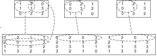
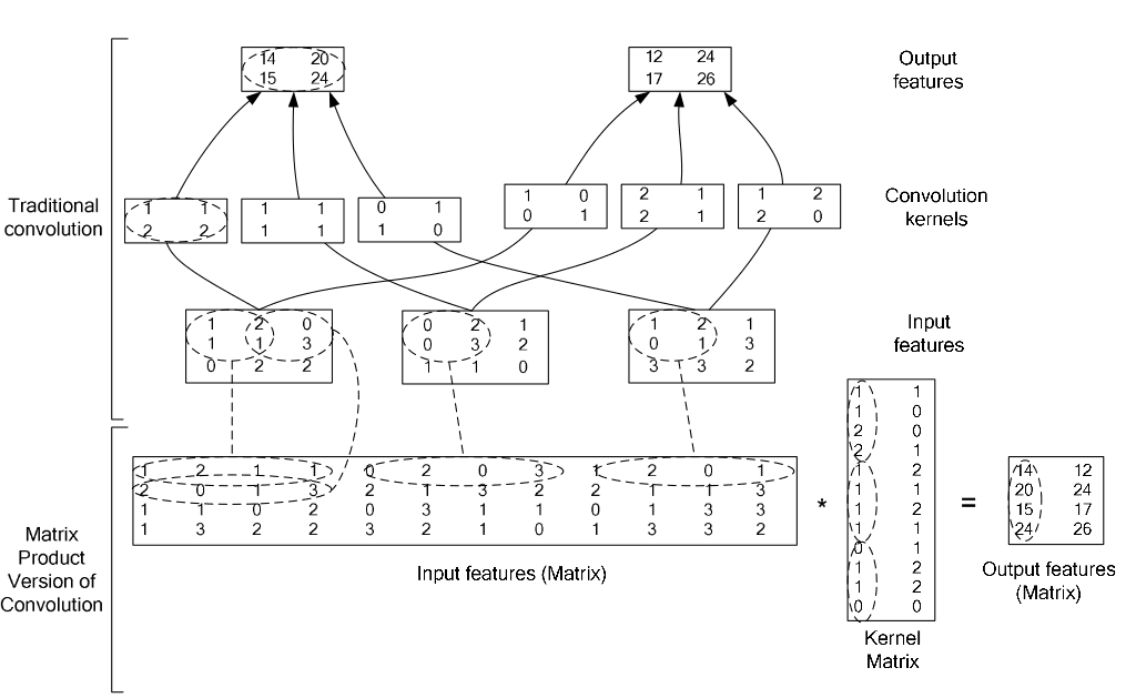
如果对matlab比较熟悉的话,就应该知道im2col是什么意思。它先将一个大矩阵,重叠地划分为多个子矩阵,对每个子矩阵序列化成向量,最后得到另外一个矩阵。
看一看图就知道了:

在caffe中,卷积运算就是先对数据进行im2col操作,再进行内积运算(inner product)。这样做,比原始的卷积操作速度更快。
看看两种卷积操作的异同:


 浙公网安备 33010602011771号