【Course】Machine learning：Week 3-logistics regression

Machine learning week3

一、 Classification and Representation

1、binary classification problem

2、Hypothesis Representation

Sigmoid Function = Logistic Function，公式如下：

\[\begin{align*}& h_\theta (x) = g ( \theta^T x ) \newline \newline& z = \theta^T x \newline& g(z) = \dfrac{1}{1 + e^{-z}}\end{align*} \]

\(h_\theta (x)\)will give us the probability that our output is 1.

\[\begin{align*}& h_\theta(x) = P(y=1 | x ; \theta) = 1 - P(y=0 | x ; \theta) \newline& P(y = 0 | x;\theta) + P(y = 1 | x ; \theta) = 1\end{align*} \]

3、Decision Boundary

决策边界:\(z = \theta^Tx=0\)

二、Logistic Regression Model

1、Cost Function

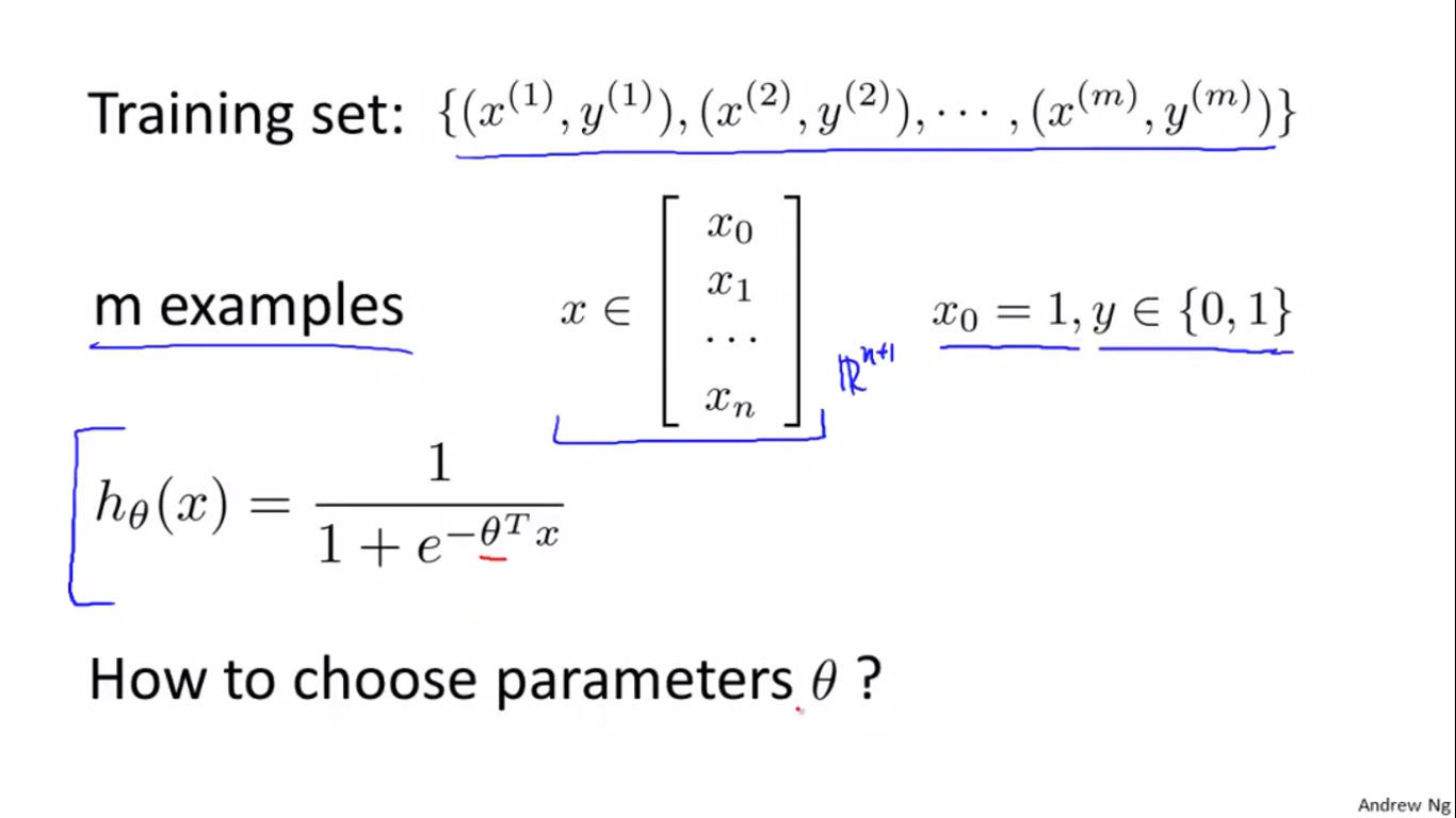
线性回归问题变成了logistic回归问题后，怎么去选择参数theta呢？

下图中，如果在logistic regression中还是用linear regression的cost function，会出现左图的cost function曲线，无法保证收敛到全局最优解。希望的是右边的convex型曲线。

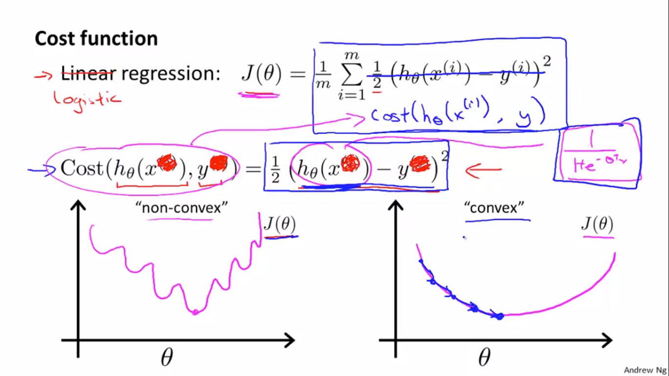
因此，logistic regression需要新的损失函数：

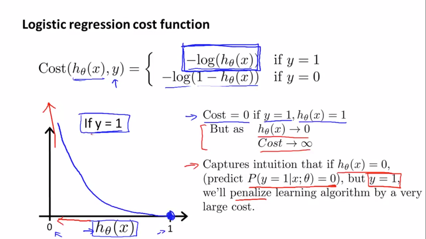
根据\(h_\theta (x)\)的定义，\(h_\theta (x)\)在[0,1]的范围内，根据log函数的曲线，就可以画出上图y=1时的损失函数\(-log(h_\theta (x))\)曲线，当y=1，\(h_\theta (x)=1\)时，证明预测值和真实值相同，Cost是等于0的。但是当\(h_\theta (x)\)-->0时，y=1时，预测错误，Cost就会很大。

下图是当y=0是的损失函数曲线：

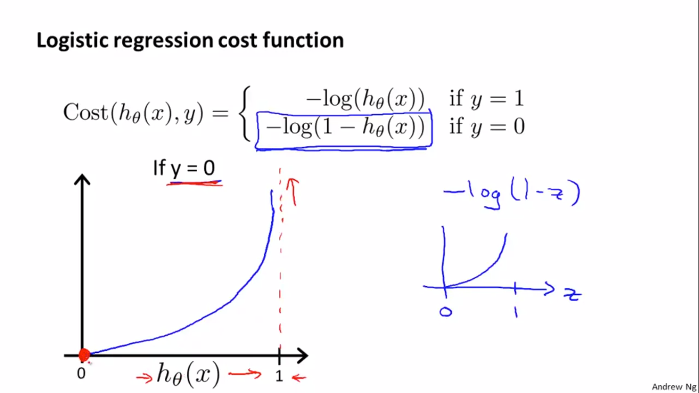
原理同y=1时，所以这个损失函数很适合于二分类的logistic regression。

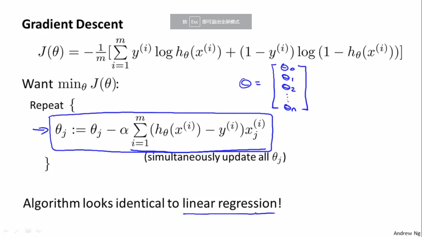
2、Simplified Cost Function and Gradient Descent

logistic regression的损失函数可以合并到一个公式里面，其梯度下降如下，Repeat部分的内容和Linear regression差不多，但损失函数\(h_\theta(x)\)是不同的。

此外，和linear regression的vectorized implementation一样，logistic regression也有vectorized implementation。公式如下：

\[\theta:=\theta-\frac{\alpha}{m} X^{T}(g(X \theta)-\vec{y}) \]

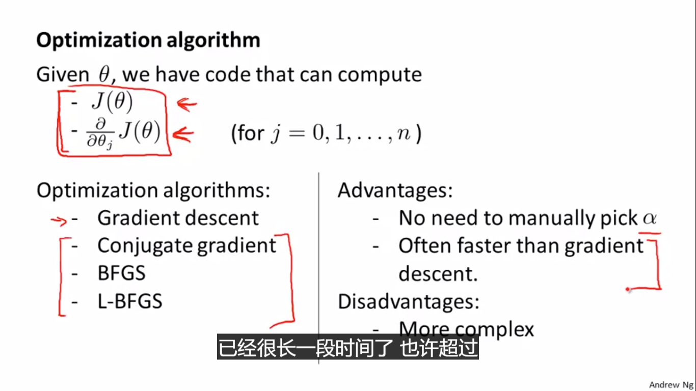
3、 Advanced Optimization

除了梯度下降，还有许多别的优化方法：

不用去追究算法的原理，目前只需要用就行。

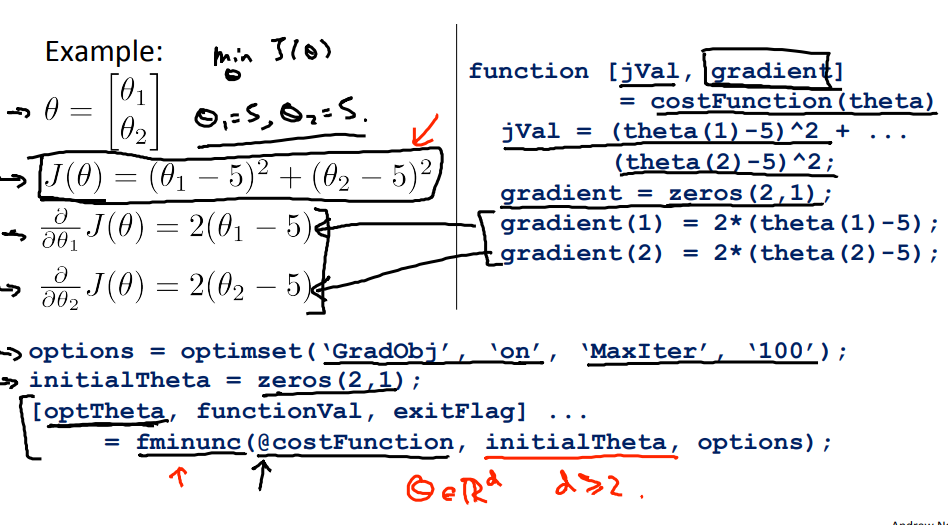
下图是调用方法：

三、Multiclass Classification

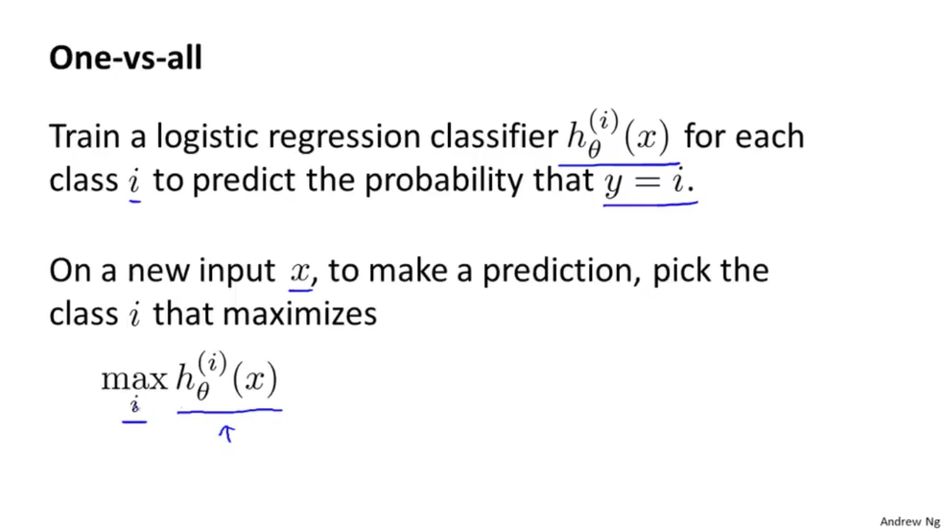
1、Multiclass Classification: One-vs-all

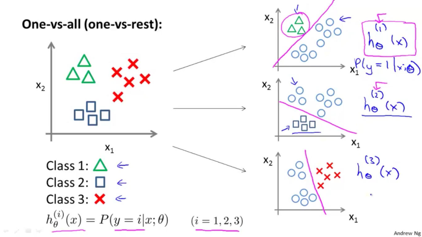
如上图，是一个一对多的分类。实际上是训练多个分类器，分别计算属于某一类的概率，再取概率最大的那个，如下图。

\[\begin{align*}& y \in \lbrace0, 1 ... n\rbrace \newline& h_\theta^{(0)}(x) = P(y = 0 | x ; \theta) \newline& h_\theta^{(1)}(x) = P(y = 1 | x ; \theta) \newline& \cdots \newline& h_\theta^{(n)}(x) = P(y = n | x ; \theta) \newline& \mathrm{prediction} = \max_i( h_\theta ^{(i)}(x) )\newline\end{align*} \]

四、Solving the Problem of Overfitting

1、The Problem of Overfitting

There are two main options to address the issue of overfitting:

1. Reduce the number of features:

• Manually select which features to keep.
• Use a model selection algorithm (studied later in the course).

2. Regularization

• Keep all the features, but reduce the magnitude of parameters \(\theta_j\).
• Regularization works well when we have a lot of slightly useful features.

2、Cost Function

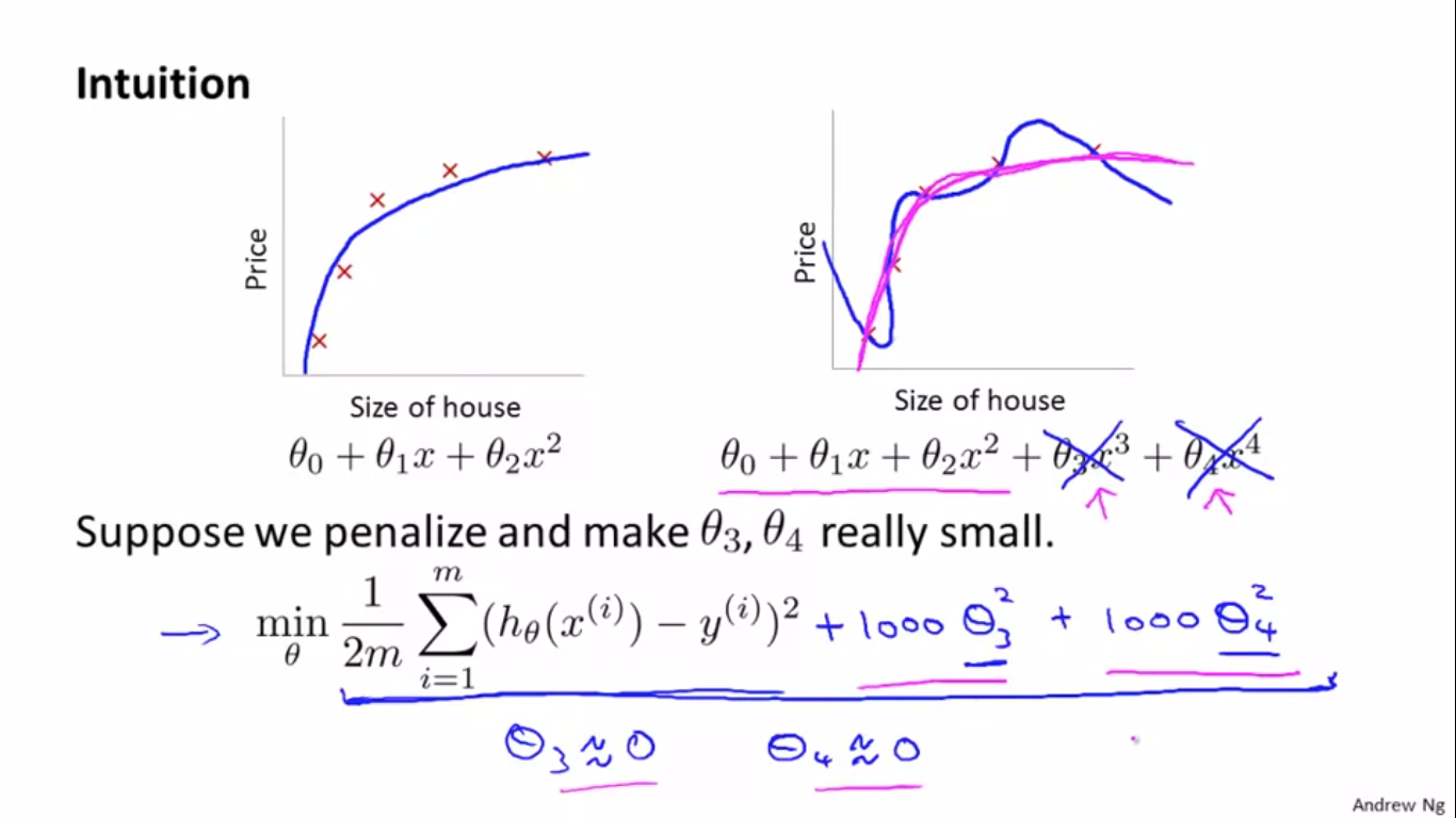
如上图所示，右图中的蓝色曲线过拟合了，因为\(\theta_3 x^3\)和\(\theta_4 x^4\)的贡献太大了，所以就想了一个办法，在最小化损失函数中加上$1000*\theta_3^2 $和\(1000*\theta_4^2\)，这样的话损失函数要想最小，那必须降低\(\theta_3\)和\(\theta_4\)的值，这样就降低了\(\theta_3 x^3\)和\(\theta_4 x^4\)的贡献，实现避免过拟合的情况。

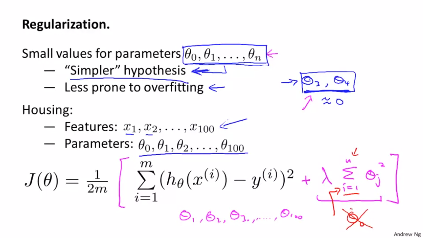
但是在实际中，当未知参数数量很多时，我们不知道惩罚哪个参数，所以，就加入一个正则项，缩小所有参数（正则项一般不包括\(\theta_0\)，包不包括差别不大，只是一种习惯），如下：

If lambda is chosen to be too large, it may smooth out the function too much and cause underfitting. 如下图：

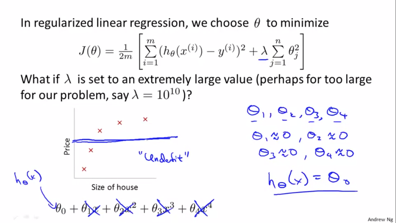
使得参数全都等于零了，所以\(h_\theta(x)=\theta_0\)，导致得到的曲线就是一条直线，出现了欠拟合（underfitting）的情况。

3、Regularized Linear Regression

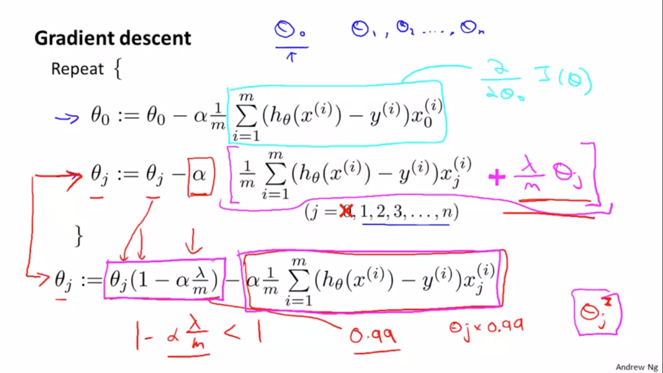
正则化后的梯度下降如上图，化简过后得到最后一排公式，直观上看比较有意思，没有正则化的线性回归的区别在于\(1-\frac{\lambda}{m}\)会是一个小于1的数，所以\(\theta_j\)会不断的去乘以一个小于一的数，后面的那一项倒是和线性回归一样。

• 正则化的正规方程（Normal Equation）：

加入正则化后的正规方程求解会变成下图所示：

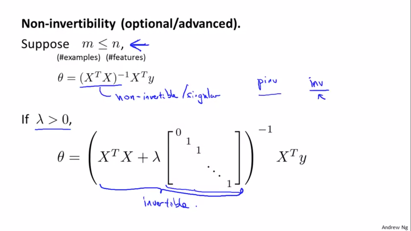
\(X^T X\)可能没有逆，虽然MATLAB/octave的pinv函数可以给出伪逆矩阵，但是求出的theta可能不太对，但是可以证明，\(X^T X+\lambda*[]\)后，\(X^T X+\lambda*[]\)就是可逆的(invertible)。

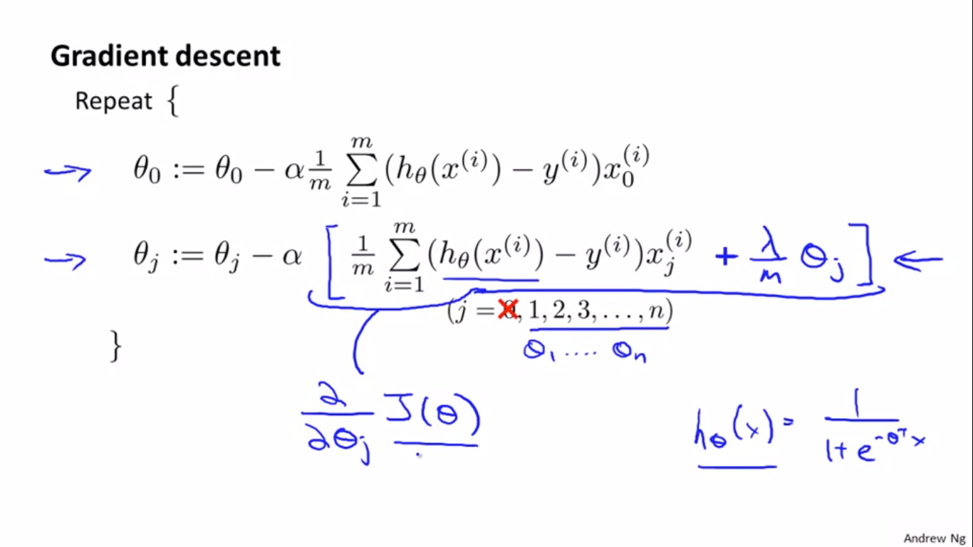
4、Regularized Logistic Regression

cost function for logistic regression was:

\[J(\theta)=-\frac{1}{m} \sum_{i=1}^{m}\left[y^{(i)} \log \left(h_{\theta}\left(x^{(i)}\right)\right)+\left(1-y^{(i)}\right) \log \left(1-h_{\theta}\left(x^{(i)}\right)\right)\right] \]

正则化后变成：

\[J(\theta)=-\frac{1}{m} \sum_{i=1}^{m}\left[y^{(i)} \log \left(h_{\theta}\left(x^{(i)}\right)\right)+\left(1-y^{(i)}\right) \log \left(1-h_{\theta}\left(x^{(i)}\right)\right)\right]+\frac{\lambda}{2 m} \sum_{j=1}^{n} \theta_{j}^{2} \]

所以，梯度下降变为：

- Advanced optimization

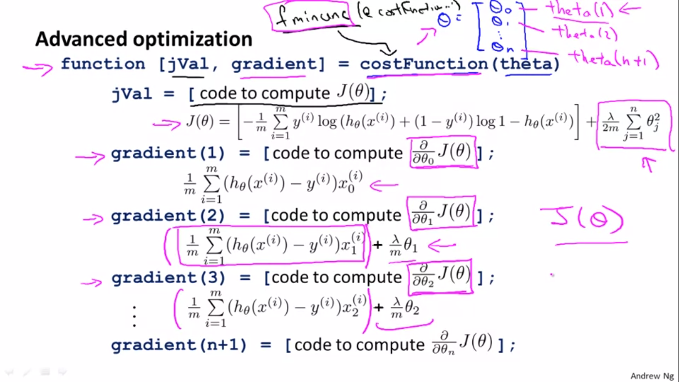
之前讲到了高级优化函数及其损失函数计算方法，在加入正则化后，变成了：

- quizzes中，这道题比较好：

最后的作业也全部完成，效果还行。