
stata数据分析学习笔记
常用命令
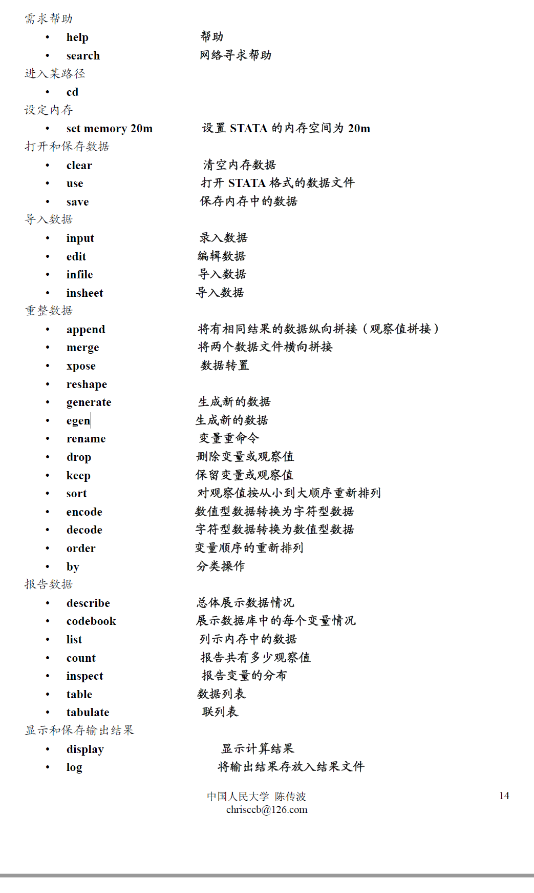
help
相当鸡肋的系统帮助页面
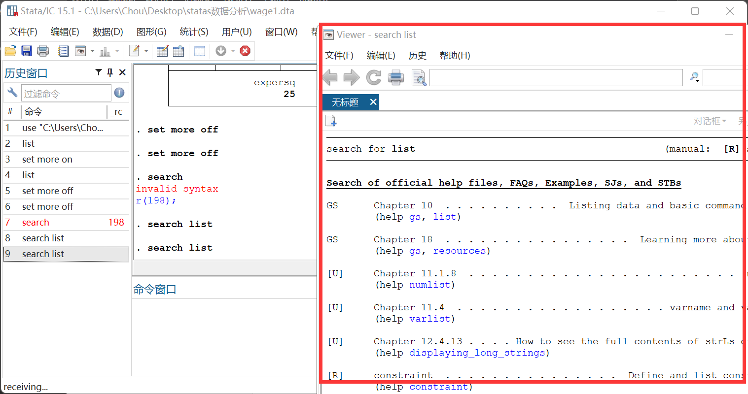
search
在网上获取帮助,鸡肋
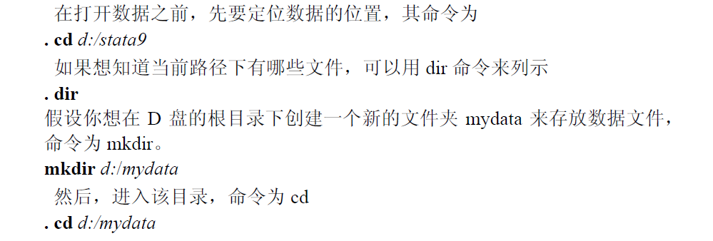
cd
设置文件路径
memory
设置内存
set memory 20m 设置STATA 的内存空间为20m
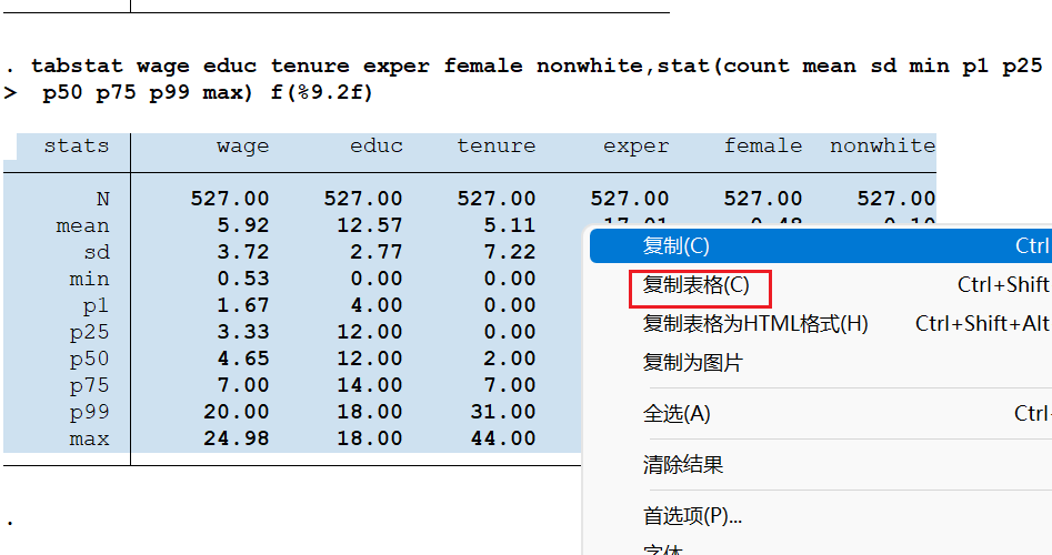
输出保留两位小数 f(%9.2f)
tabstat wage educ tenure exper,stat(count mean sd min p1 p25 p50 p75 p99 max) f(%9.2f)
🤔输出结果
第一种 右键
第二种 asdoc
ssc install asdoc, replace
asdoc xxxx
打开和保存数据
• clear 清空内存数据
• use 打开STATA 格式的数据文件
• save 保存内存中的数据
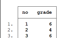
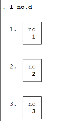
input
录入数据
input x 录入列名为x的数据
end
结束输入
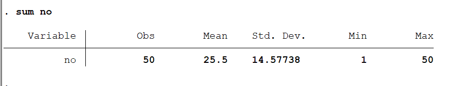
sum
观察值个数,平均值,方差,最小值和最大值
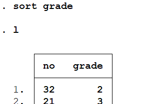
sort
sort grade 排序(按grade从低到高)
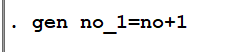
gen
生成新的变量
egen
生成新的数据
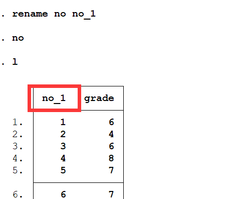
rename
重命名变量名
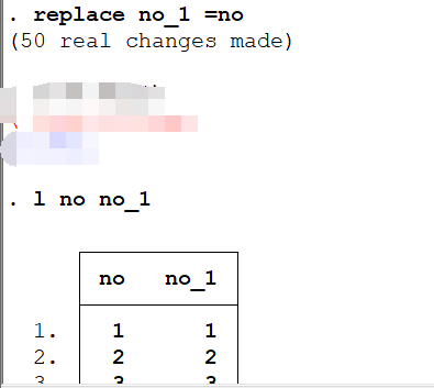
replace
直接改变原变量的赋值
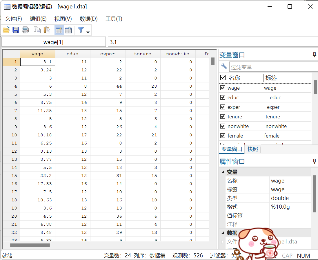
edit
编辑数据,输入
edit会打开数据编辑器
display
显示计算结果
disp normal(1)结果是0.5
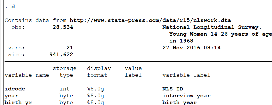
describ
d 直接输入d
describ 命令显示数据集的属性信息
set more off/on
是否显示全部数据on 意思是不显示全部
在列示1 到1000 之前,若先设置set more off,则屏幕不停止;反之set more on 会使显示停止。
clear
清除内存中原有内容,不把你的数据删了(慎用)
drop
drop_all删除全部数据,效果同clear
drop x 删除x这一列数据
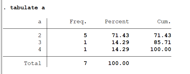
tabulate
频数分析
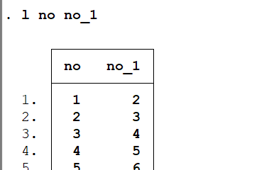
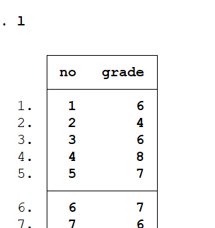
list
list x显示示x列的数据
list 显示全部数据
暂时没用到的
• infile 导入数据
• insheet 导入数据
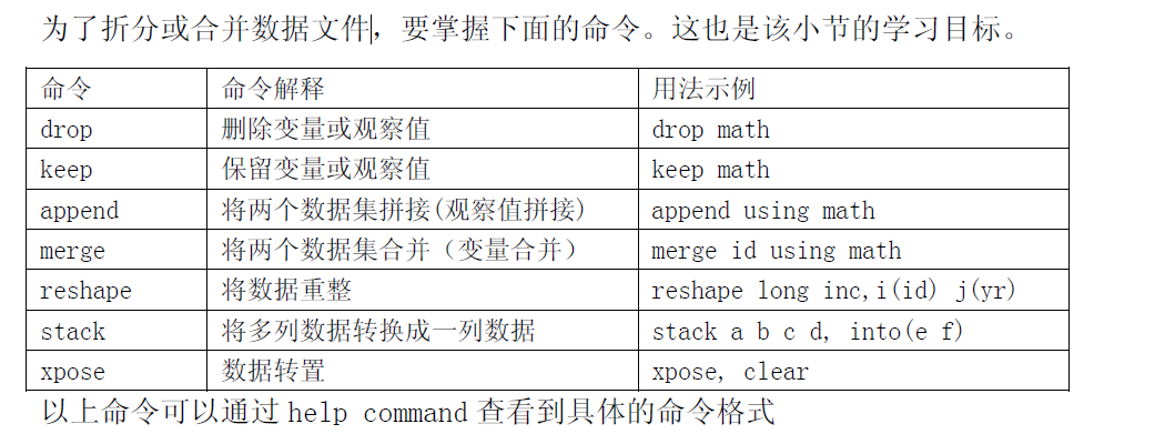
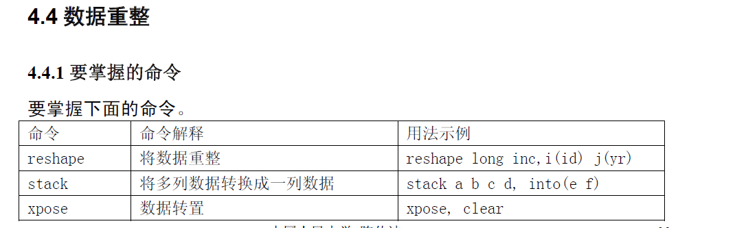
重整数据
• append 将有相同结果的数据纵向拼接(观察值拼接)
• merge 将两个数据文件横向拼接
• xpose 数据转置
• reshape
• generate 生成新的数据
• egen 生成新的数据
• rename 变量重命令
• drop 删除变量或观察值
• keep 保留变量或观察值
• sort 对观察值按从小到大顺序重新排列
• encode 数值型数据转换为字符型数据
• decode 字符型数据转换为数值型数据
• order 变量顺序的重新排列
• by 分类操作
报告数据
• describe 总体展示数据情况
• codebook 展示数据库中的每个变量情况
• list 列示内存中的数据
• count 报告共有多少观察值
• inspect 报告变量的分布
• table 数据列表
• tabulate 联列表
显示和保存输出结果
• log 将输出结果存放入结果文件
命令汇总
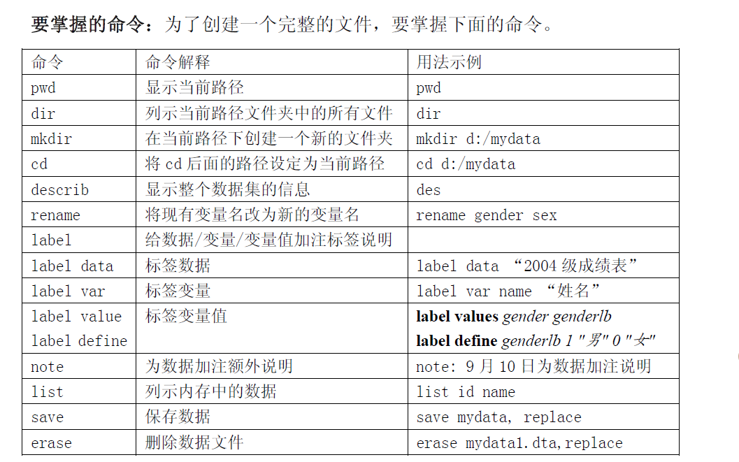
1.创建完整文件
2.才拆分合并数据
3.数据重组
变量的省略规则
只要不引起歧义,命令可以尽量只写前几个字母。如summarize 只需要前两个字母su;而
list 只需要写第一个字母l。在帮助文件中,命令下面有小划线,该线表明了命令可以省略
到什么程度。如
list [varlist] [if] [in] [, options]
summarize [varlist] [if] [in] [weight] [, options]
变量命名规则
和Python差不多
除以下字符不能用作变量名外,任何字母、字母与数字(单独的数字也不允许)组合均可用做
变量名:_all _b byte _coef _cons double float if in int long _n _N _pi _pred _rc _se _skip using with
基本要求如下:
- 第一个字元可以是英文字母或, 但不能是数字;
- 最多只能包括32 个英文字母、数字或下划线;
- 由于STATA 保留了很多以“ _“开头的内部变量,所以最好不要用为第一个字元来定义变量。
命令语句
command
command [=exp] [if exp] [in range] [weight] [, options]
注:[ ]表示可有可无的项,显然只有command 是必不可少的
. cd d:/stata9
. use auto, clear //打开美国汽车数据文件auto.dta,后面的clear 表示先清除内
存中可能存在的数据集
. summarize /*很多命令可单独使用,单独使用时,一般是对所有变量进
行操作,等价于后面加上代表所有变量的_all。 */
. summarize _all //注意到该命令输出结果与上一个命令完全一样
. sum //与前一命令等价,sum 为summarize 的略写
. su // su 是summarize 的最简化略写,不能再简化为s
. s //简写前提是不引起混淆。执行这个命令将出现错误信息
varlist
command [varlist] [=exp] [if exp] [in range] [weight] [, options]
varlist 表示一个变量,或者多个变量,多个变量之间用空格隔开。
. cd d:/stata9
. use auto, clear
by varlist 分类操作
[by varlist:] command [varlist] [=exp] [if exp] [in range] [weight] [, options]
sort foreign //按国产车和进口车排序
by foreign: sum price weight注意必须先sort foreign 这个变量 才能 by foreign先排序再分类
赋值及运算=exp
[by varlist:] command [varlist] [=exp] [if exp] [in range] [weight] [, options]
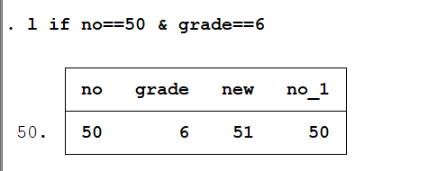
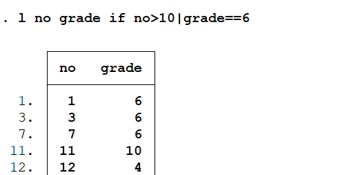
|或
&和
<> 大于小于
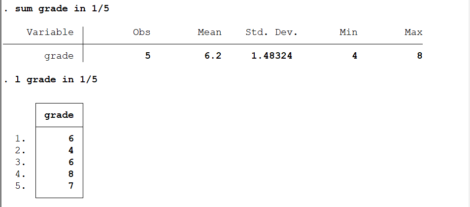
范围筛选in range
[by varlist:] command [varlist] [=exp] [if exp] [in range] [weight] [, options]
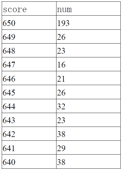
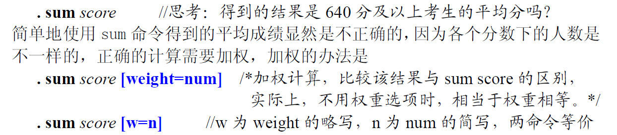
加权weight
其他可选项,options
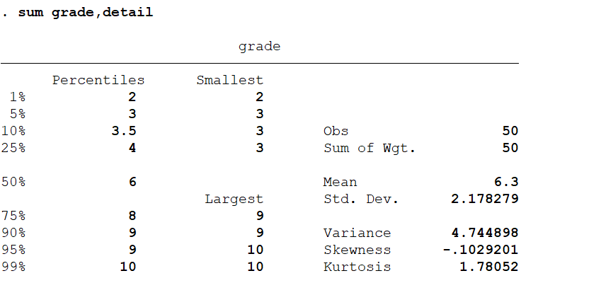
sum grade
Variable | Obs Mean Std. Dev. Min Max
-------------+---------------------------------------------------------
grade | 50 6.3 2.178279 2 10
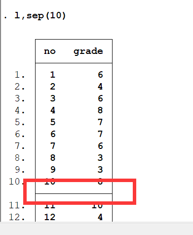
detail可以显示细节的内容
sep(x)每x行添加一个横线
数据类型转化
字符型转化成数值型:destring
数值型转化为字符型:tostring
数据显示格式:format
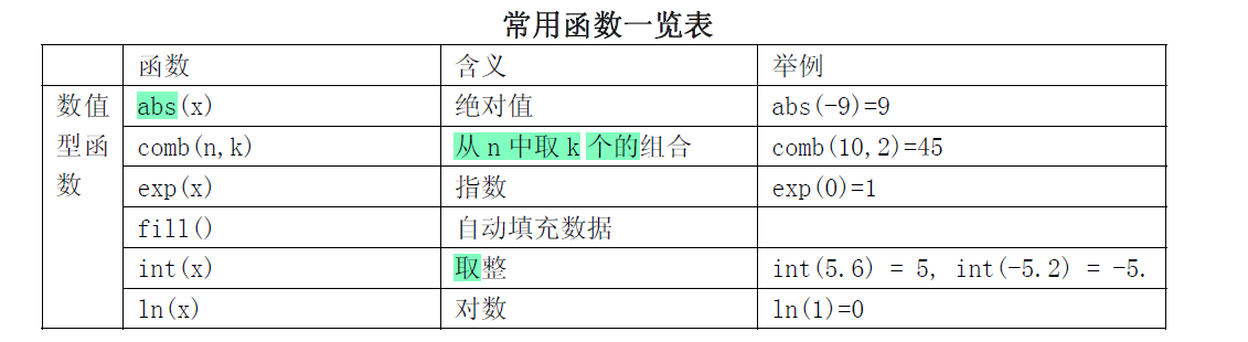
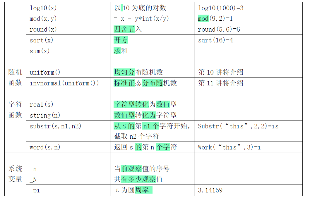
stata函数
正态分布、F分布、卡方分布的概率密度和分位数
normal 正态分布概率密度
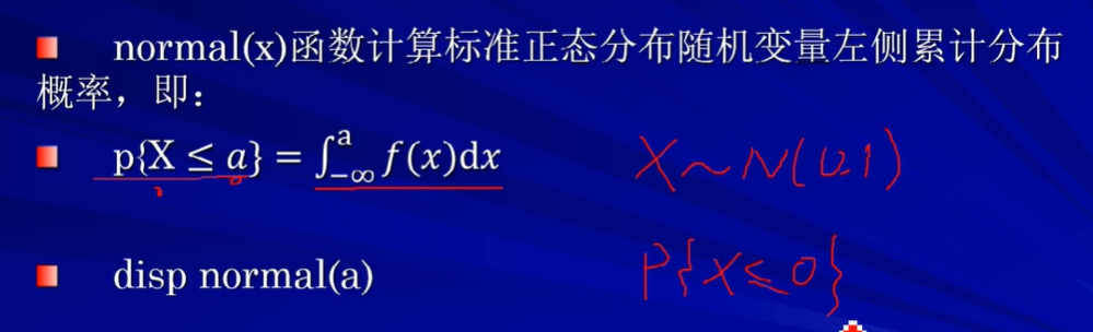
invnormal正态分布分位数

t分布概率密度
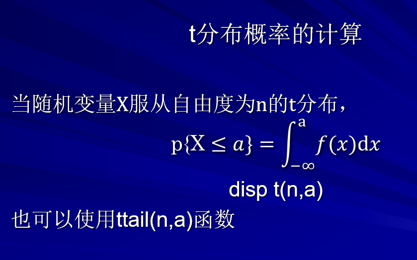
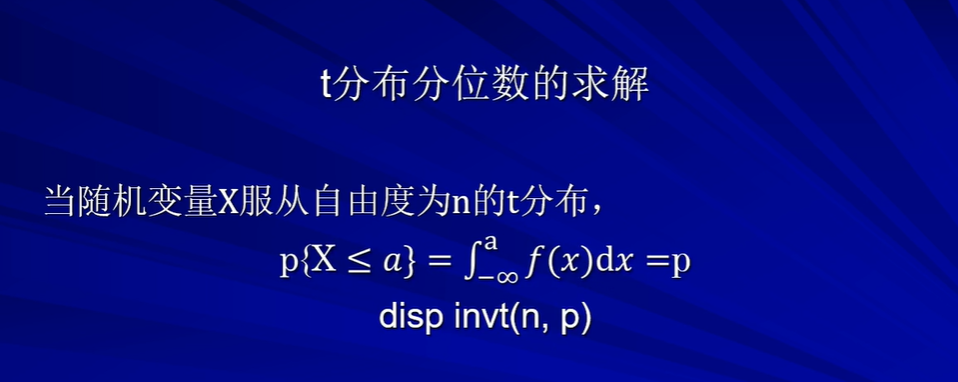
t分布分位数计算
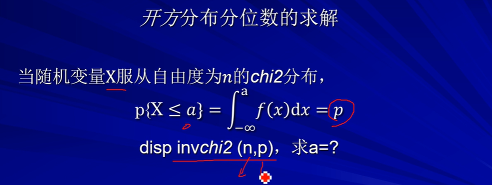
卡方分布概率密度

卡方分布分位数
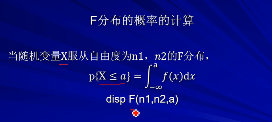
F分布概率密度
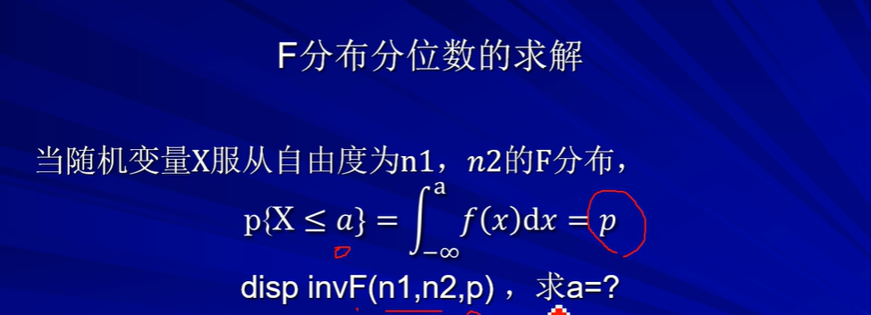
F分布分位数
区间估计(补充知识)
一、区间估计
(一)命令
- 直接命令为:cii 样本量 样本均数 样本标准差, level(99)
例如,变量wage的描述统计如下:
Variable Obs Mean Std. Dev.
wage 526 5.896103 3.693086
则可以运用cii命令直接构建其置信区间:
cii 526 5.9 3.7, level(99)
注意:level(99)中的99表示置信概率为99%,该值可以根据需要改变。
- 原始数据的命令:ci 变量,level(99)
如当前环境中有变量wage(直接建立或输入),则可以运用ci命令构造其置信区间:
ci wage,level(99
假设检验(补充)
原假设一般是研究者怀疑的假设
备择假设是研究者想收集证据予以支持的的假设
传统假设检验
一般不用
(❗待完善)p值假设检验
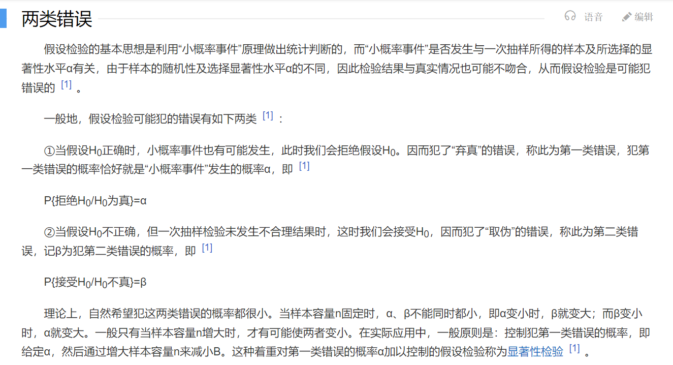
1.显著性水平p值:检验者可以容忍的犯第一类错误的概率
2.第一类错误 :H0真 但判断H0假
3.一般样本容量n>30都认为是大样本,可以按正态分布计算
4.较小的p值是拒绝原假设H0的证据
(一)直接命令为:
ttesti 样本量 样本均数 样本标准差 (待检验的总体均数)
(二)原始数据的命令:
ttest 变量名 = (待检验的总体均数)使用说明:如当前环境中有变量wage(直接建立或输入),则可以运用ci命令构造其置信区间:
ttest wage=6
变量分布形态和假设检验
分布状况
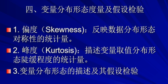
偏度
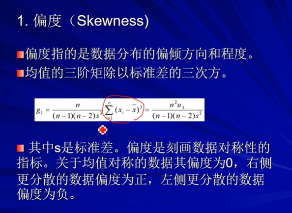
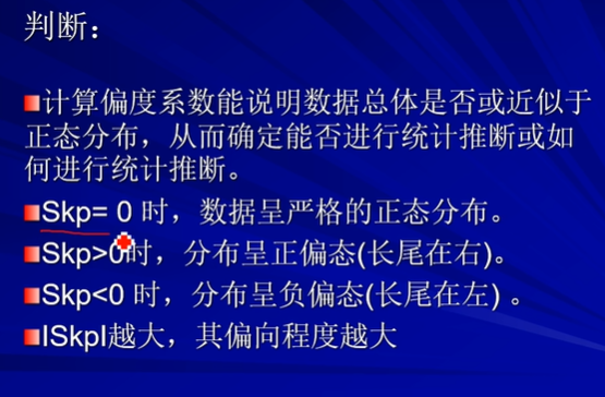
Skewness 偏度
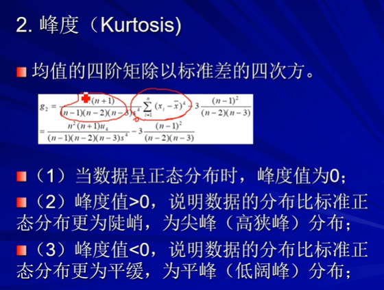
Kurtosis 峰度
su wage,detail
tabstat wage,stat(count skewness kurtosis )
假设检验


sktest wage aaa bb cc
参数假设检验
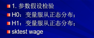
sktest wage
skwilk wage
H0:变量服从正态分布
H1:变量不服从正态分布
输入sktest wage/skwilk可以得到pr(skewness)偏度、 pr(kurtosis)峰度、 prob>chi2这个值很小的话就代表不符合原假设的正态分布
非参数的假设检验
signrank before=after
signtest before=after
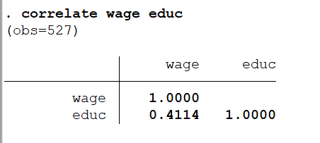
相关系数计算和检验
相关性计算
相关系数0.3-0.8是弱相关性
0.8以上强相关
0.3以下无相关性


1.person


correlate a b c
pwcorr a b c,sig star(0.05)
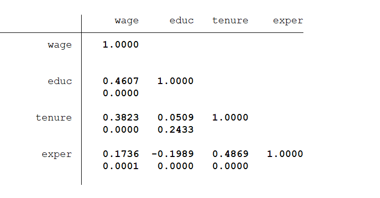
2.spearman
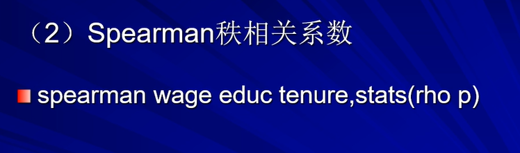
spearman a b c,stats(rho p)
rho:相关系数
p:假设检验
3.kendall
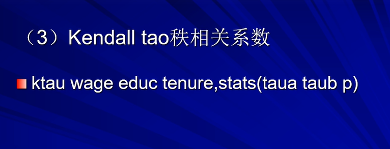
ktau wage educ tenure exper,stats(taua taub p)
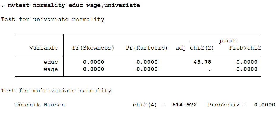
多变量分布检查(了解)
多变量联合正态分布

mvtest normality a b,univariate

单变量和多变量的统计分析
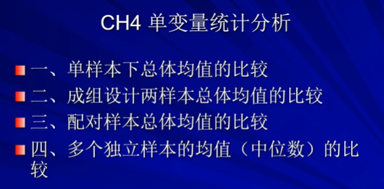
单样本下总体均值的比较
单样本总体均值的比较是根据样本数据检验总体均值与某个特定数之间是否存在显著差异
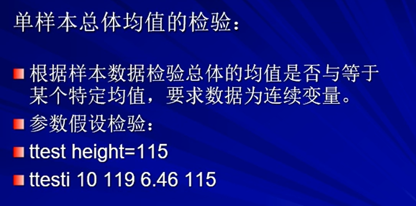
ttesti 样本量 样本均数 样本标准差 (待检验的总体均数)
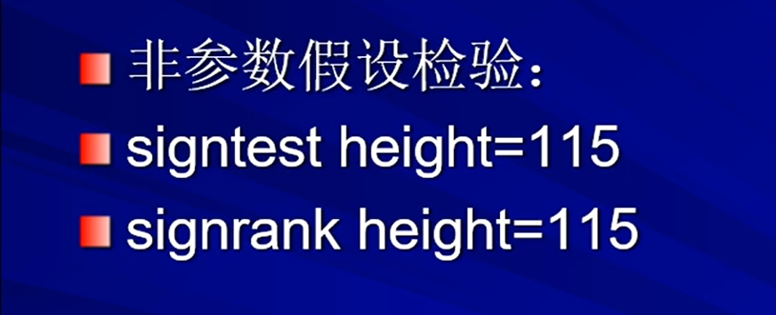
signtest height=115
signrank height=115
❗如果差别比较大按signrank为主
参数型成组设计两样本总体均值的比较
待检验数据符合正态分布
样本数据:
| jiaoqu | city |
|---|---|
| 108 | 110 |
| 112 | 123 |
| 129 | 109 |
| 131 | 130 |
| 118 | 125 |
| 121 | 120 |
| 115 | 119 |
| 110 | 118 |
| 124 | 115 |
| 120 | 121 |
| 116 | 117 |
| 120 | 125 |
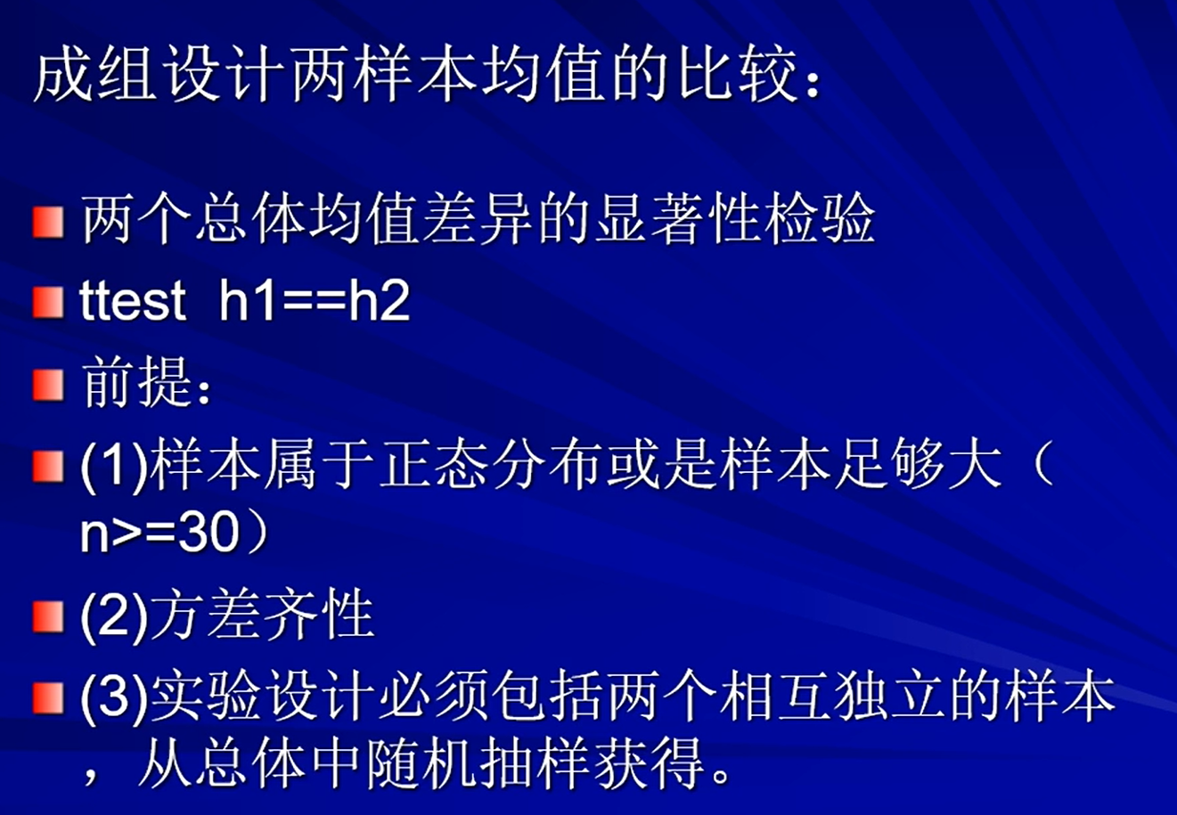
首先提出假设:
H0:城区和郊区男童身高相等
H1:城区和郊区男童身高不相等
第一步.需要先对每组变量进行正态分布的假设检验
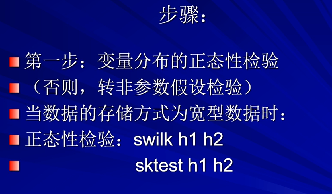
swilk jiaoqu city
sktest jiaoqu city
根据p值得大小判断是否符合正态分布越接近1说明越符合正态分布
第二步.方差齐性检验
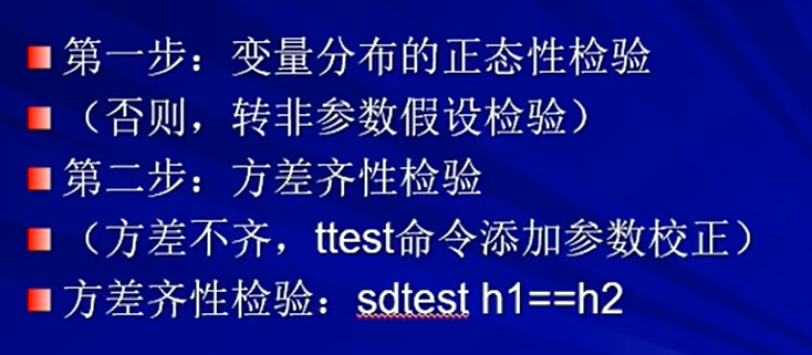
H0:两组数据方差相等
H1:两组数据方差不相等
sdtest jiaoqu==city
第三步.前两步都满足的情况下

ttest jiaoqu==city
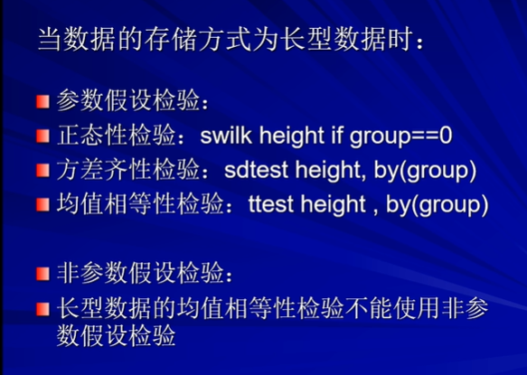
非参数性总体均值比较
如果参数均值比较第一步正态检验 不通过 就用非参数型
同样要进行方差齐性检验sdtest

signrank before=after
signtest before=after
注意:
多个独立样本的均值(中位数)的比较
参数的看方差分析
非参数的:


kwallis wage,by(numdep)
方差分析-单因素(补充)
概念
检验多个总体均值是否相等
自变量:定类2个及以上
因变量:连续变量
主要用于随机化试验设计
提假设
H0:u1=u2=u3=u4
H1:u1,u2,u3,u4不全相等
总变动SST(误差):所有样本观测值与总平均值的偏离的 平方的和
1.总误差产生的原因:
组内变动SSE——随机误差 = 组内样本与组平均之差的平方和
组间变动SSA——系统误差 = 每组平均数与总平均之差的平方和
方差分析的基本思想和原理——方差的比较
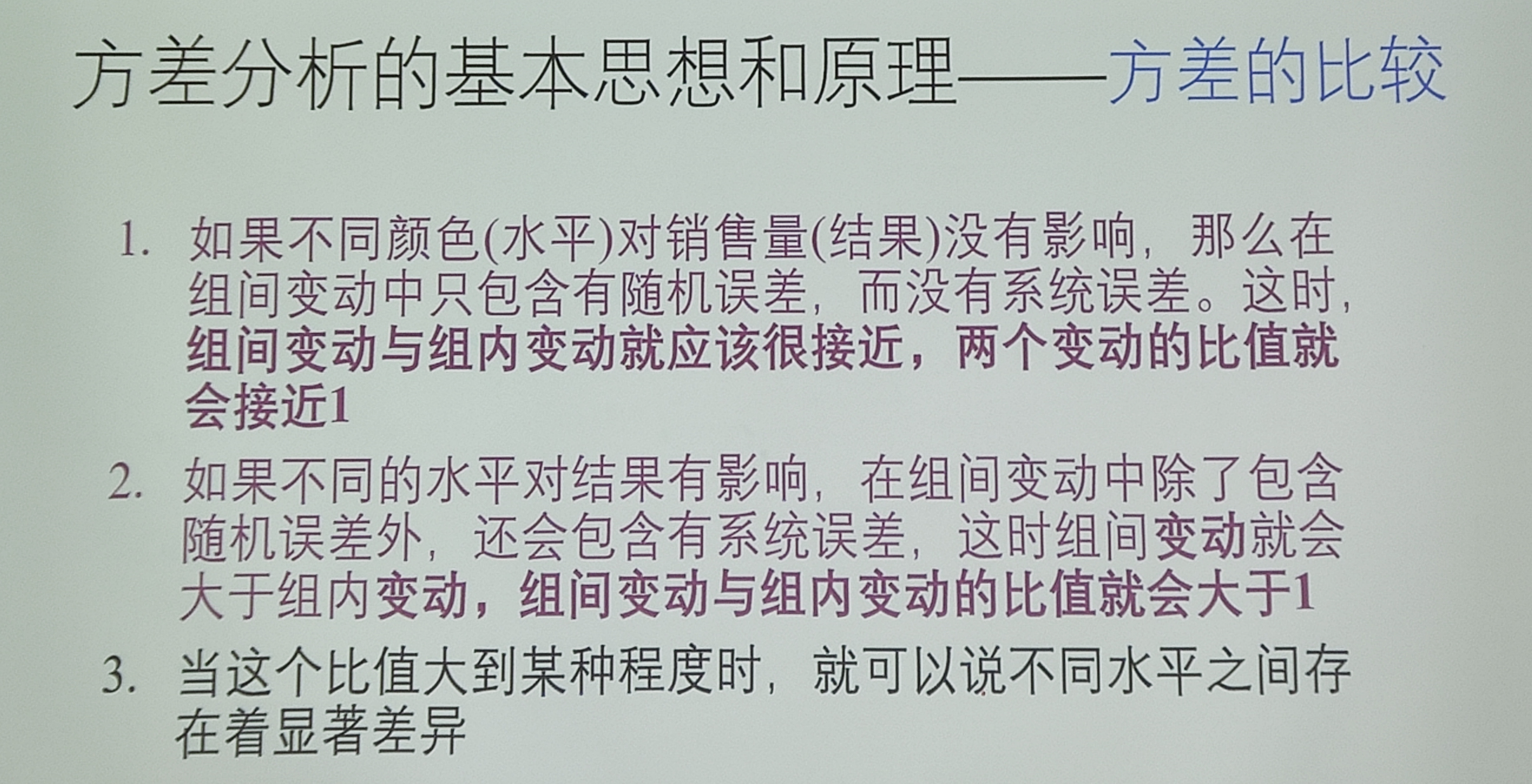
计算步骤
计算组内平均
计算组间平均
计算总平均
就算总变动SST
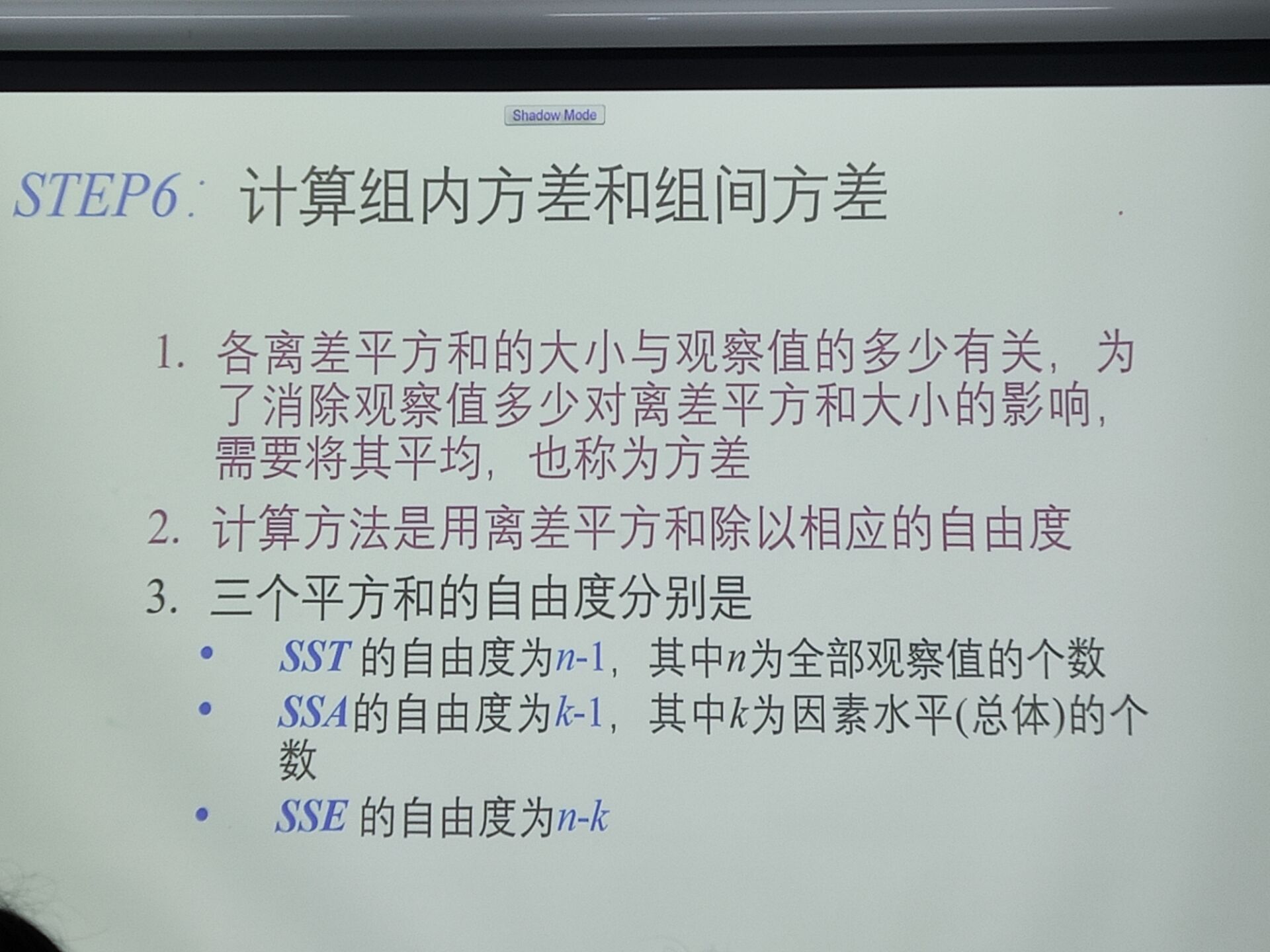
计算组内变动SSE和组间变动SSA
stata 处理方法
输入格式:
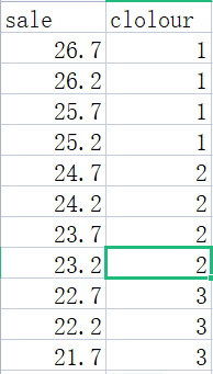
oneway sale colour,tabulate
anova sale colour
partial ss 组间变动
df分子自由度 F(3,16,10.46)
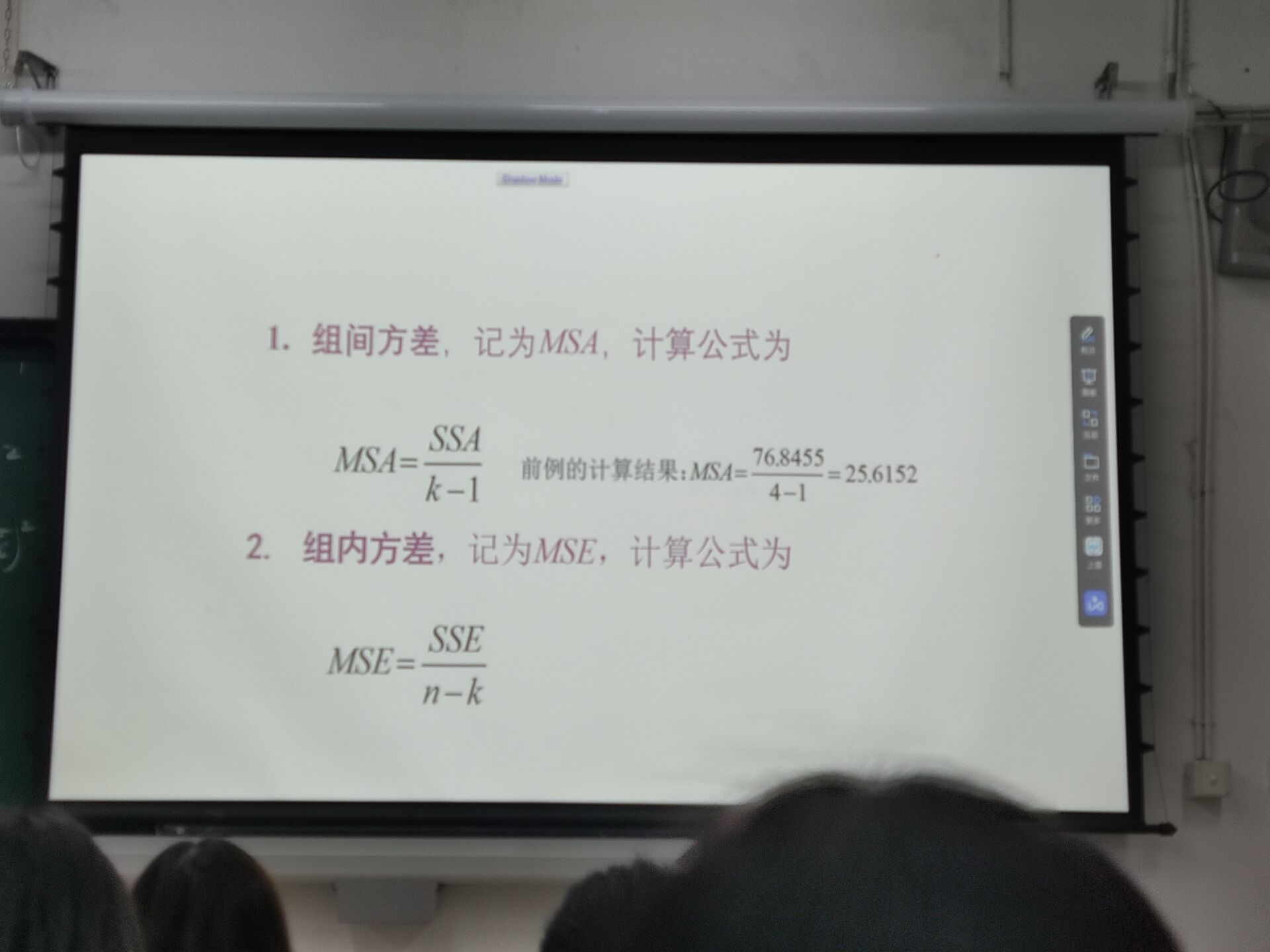
MS =partial ss/df
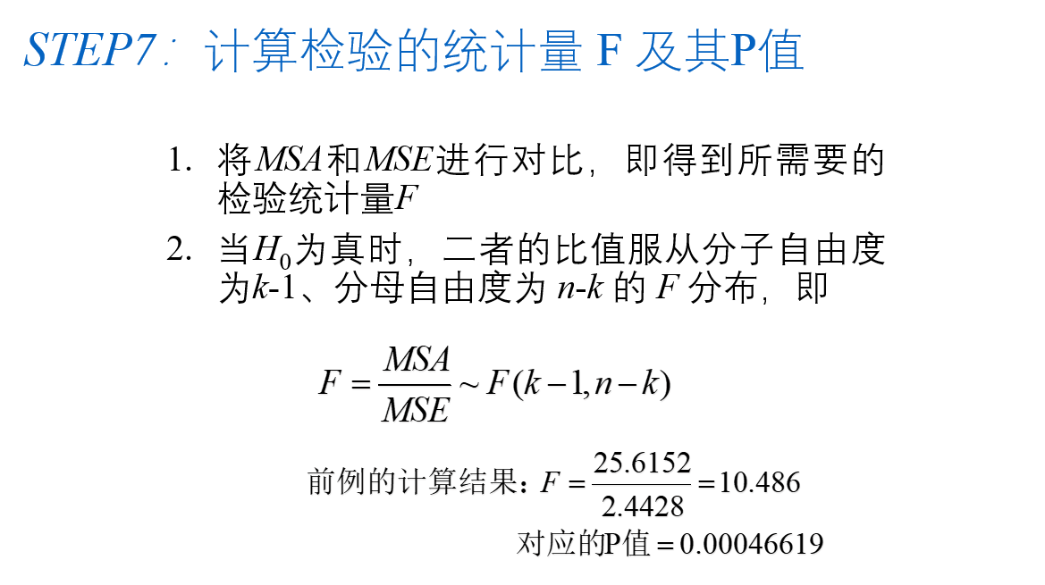
F 检验量
方差分析-双因素
residual误差项
stata绘图
基本命令
graph-command (plot-command, plot-options) (plot-command , plot-options) , graph-options
或者
graph-command plot-command,plot-options || plot-command , plot-options || , graph-options
graph-command定义图的类型,plot-command 定义曲线类型,同一个图中如果有多条曲线可以用括号分开,也可以用“||”分开,曲线有其自身的选项,而整个图也有其选项。例如twoway为graph-command中的命令之一,而scatter为plot-command中的命令之一。
STATA 提供各种曲线类型,包括点(scatter)、线(line)、面(area),直方图(histogram)、条形图(bar)、饼图(pie)、函数曲线(function)以及矩阵图(matrix)等。对时间序列数据有以ts 开头的一系列特殊命令,如tsline。还有一类是对双变量的回归拟合图(lfit、qfit 、lowess)等。
绘图常用命令
标题项: title(xxx)
图的副标题:subtitle(xxx)
坐标轴格式
1.默认有坐标轴、刻度线
2.无坐标轴格式
yscale(off)
xscale(off)
plotregion(style(none))
3.无坐标轴,有刻度格式
plotregion(style(none))
yscale(noline)
xscale(noline)
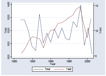
4.双坐标轴格式
line rainfall yield year //该命令等价于
tw (line rainfall year)
(line yield year)
5.坐标轴标题
纵坐标标题:ytitle()
横坐标标题:xtitle()
6.坐标轴刻度
左纵坐标刻度:ytick()
下横坐标刻度:xtick()
7.任意水平线与垂直线:yline()与xline()
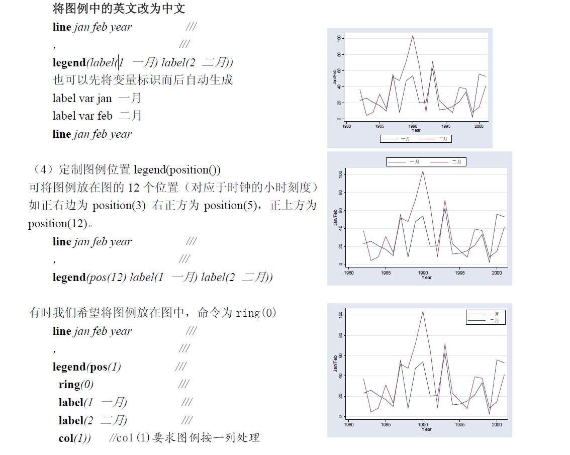
8.图例legend()
legend(off)
定制图例:
9.脚注:note()
常用的图
我会用stata作图,替换工具很多比如spss
    Command               Description
    --------------------------------------------------------------------
    histogram             histograms直方图,经验分布图
    lfit                  拟合曲线
    symplot               symmetry plots
    quantile              quantile plots
    qnorm                 quantile-normal plots
    pnorm                 normal probability plots, standardized
    qchi                  chi-squared quantile plots
    pchi                  chi-squared probability plots
    qqplot                quantile-quantile plots

    gladder               ladder-of-powers plots
    qladder               ladder-of-powers quantiles

    spikeplot             spike plots and rootograms
    dotplot               means or medians by group
    sunflower             density-distribution sunflower plots
    --------------------------------------------------------------------
多个图 twoway (画图命令1) (画图命令2) by(如果要分类)
单个图 histogram xxx
经验分布图
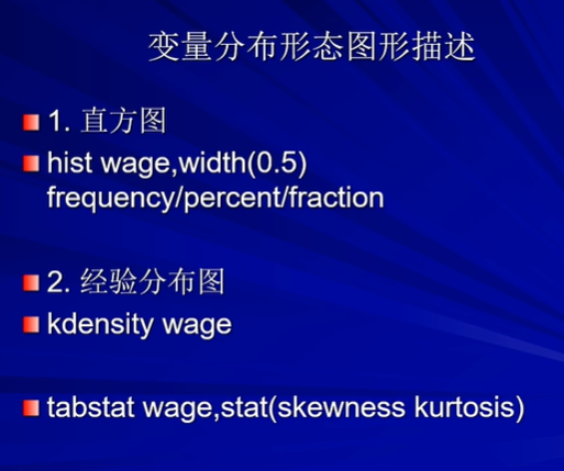
histogram xxx,width(0.5)
描述性统计的计算


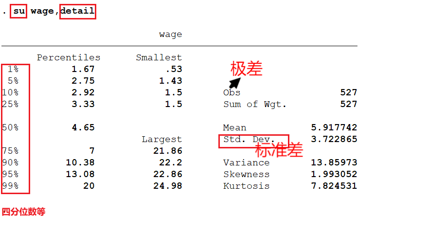
分位数(四分位数等)、标准差、极差
su wage,detail
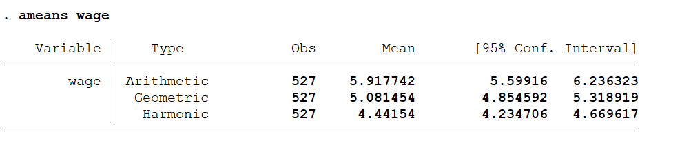
算术平均数、集合平均数、调和平均数
ameans wage
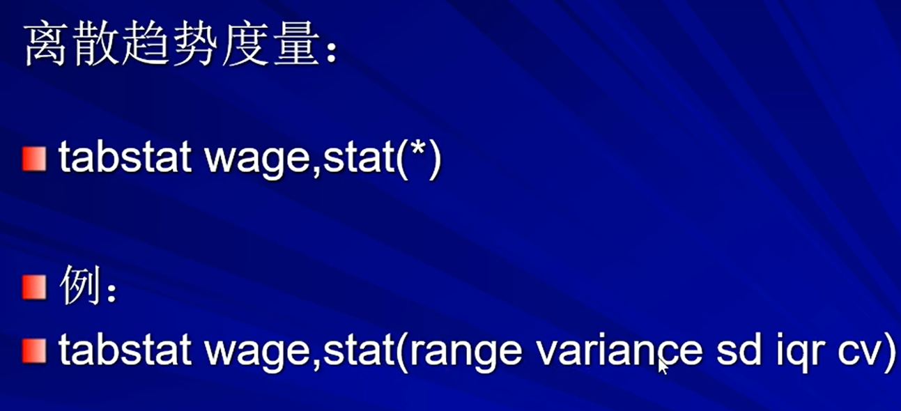
离散趋势度量:
tabstat wage,stat(range variance sd iqr cv)
range极差
variance方差
sd标准差
iqr四分位差 75%分为数-25%分位数
cv 离散系数 = 标准差Std. Dev./均值mean
通过help tabstat查看更多
变量保存
return ls
su sale if colour==1

 浙公网安备 33010602011771号