(模拟)布料仿真的基本方法
本文禁止转载
B站:Heskey0
布料仿真的两大类方法:
1. Mass-Spring Damper Model
Pros:
- It is derived from natural tendency and is easier to implement
Cons:
- The model is not derived from theory or observations which makes it less accurate.
- It has too much of coupling among the springs.
- Setting spring constant values to obtain desired effect is difficult
2. Elasticity-Model
By considering the surface of the cloth and integrating all the energy functions a more accurate model was designed called Elasticity Model which includes the following properties:
- There exists a resistance in triangles and edges while making changes to their size. So energy is required if we want to compress or expand them.
- Bending is resisted by the edges. So energy is required if two adjacent faces needs to be bent.
- Deformation is resisted by triangle. So energy is required in deforming or shearing a triangle.
Chapter 1. 中科大
2021年(第九届)中国科学技术大学《计算机图形学前沿》暑期课程_哔哩哔哩_bilibili
1.1 An overview of the cloth simulation
Cloth simulation in known to be slow:
- Dynamics Solver (40% of the total cost)
- High resolution
- High nonlinearity: 布料抗拉伸却易弯曲
- High stiffness
- Collision Handling (60% of the total cost)
- Collision detection
- Collision response
1.1.1 时间积分
Backward Euler Integration/ implicit Euler:
可推出:
上式等价于一个优化问题(对下面的\(F(X)\)求导即可证明):
重新构建一个Nonlinear optimization:(也可以构建关于 \(v^{t+\Delta t}\) 的优化问题)
where: (加号左边是kinetic energy,右边是potential energy)
\[F(x)=\frac1{2\Delta t^2}(x-\bar x)^TM(x-\bar x)+E(x) \]and
\[\bar x=x^t+\Delta tv^t \]
1.1.2 Collision Handing
discrete collision handling:
- 只保证每一个状态都处于安全状态
- 不保证是否发生碰撞
碰撞是一个约束:
where:
- \(\Omega\): intersection-free region
continuous collision handling:
1.2 (basic method) Popular methods for real-time cloth simulation
1.2.1 非线性优化的套路
非线性优化的solver,通常是满足以下形式:
An iterative nonlinear solver typically has the form: (with certain acceleration methods)
where:
- step size: \(\alpha\)
- matrix: \(A\)
- gradient: \({\part F(x^{k})}/{\part x}\)
1.2.2 Newton-Raphson
Newton-Raphson中,\(A\) 是一个Hessian matrix:
Pros (优点):
- 2rd-order convergence rate. (单位时间内,error=error/2)
Cons (缺点):
-
How to solve \(A^{-1}\) 或者说 \(A^{-1}f\) ?
- Direct, Iterative (PCG)
-
It can fail to converge if \(x\) is far from the solution
- small step size
- Hessian must be enforced to be positive define
- 很多迭代法要求矩阵是positive define的
Newton-Raphson方法的应用:
Papers:
- (1996) Large step on cloth simulation: 只用了一次Newton iteration
Marvelous Designer (mostly CPU, has GPU)
- 一次Newton iteration solved by limited PCG iterations
1.2.3 Gradient Descent
Gradient Descent中,\(A\) 是一个identity matrix:
Pros:
- Very GPU friendly
- Very simple
Cons:
- 1st-order convergence rate (收敛很慢)
- No simulator uses this as it is.
1.2.4 Projective Dynamics
Projective Dynamics中,\(A\) 是一个Constant smoothing matrix:
Pros:
- Fast on CPUs, since \(C\) can be pre-factorized. (在CPU上对 \(C\) 做预分解)
- Fast convergence in the first few iterations
- Intuitively, the use of \(C\) quickly smooths out some low-frequency errors.
Cons:
- Not GPU-friendly
- 矩阵的inverse,通常不是sparse matrix。会导致矩阵乘法效率慢
- 1st-order convergence rate: slow convergence overall. (一开始收敛快,然后像gradient descent一样收敛慢)
1.2.5 Diagonal Hessian
(sig asia 2015)Diagonal Hessian中,\(A\) 是一个Hessian matrix的diagonal matrix:
Pros:
- Converges faster than gradient descent
- GPU friendly
Cons:
- Still does not converge that fast
1.3 (Acceleration) Popular methods for real-time cloth simulation
有了非线性算法,还需要加速算法,如:
- (2015) Chebyshev
- (2015) Nesterov
- (2018) Anderson
- (2017) L-BFGS
Only Chebyshev is GPU-friendly. Multiscale acceleration is also effective
1.3.1 Chebyshev
算法:
-
For \(k=0,...,K\)
-
\[x^{(k+1)}=x^k-\alpha^{(k+1)}(A^{(k+1)})^{-1}\frac{\part F(x^{k})}{\part x} \]
-
if \(k==0\) then \(\omega=1\)
-
if \(k==1\) then \(\omega=2/(2-\rho)^2\)
-
if \(k>1\) then \(\omega=4/(4-\rho^2\omega)\)
-
\(x^{(k+1)}=\omega x^{(k+1)}+(1-\omega)x^{(k-1)}\)
-
\(\rho\) is the spectral radius, i.e. the estimation of the residual error decreasing rate
For example:
- 某次迭代,error=error*0.99,则 \(\rho\approx 0.99\)
推荐套路:
- CPU:
- Projective dynamics followed by Newton-Raphson
- GPU:
- Chebyshev + Diagonal Hessian
- Newton-Raphson with PCG
1.4 The remaining topics
1.4.1 Position-Based Dynamics
不去解数学问题:
而是通过直接将两个顶点拉近,修改顶点的位置(非物理)
Pros:
- No physical quantities
- Everything on GPU shared memory, fast! (NVcloth)
- 当顶点少的时候,直接将顶点数据放到shared memory中,访问快
Cons:
- No physical meaning
- Not scalable. (Shared memory is only 16kB)
- vertex多的时候,效率会显著下降
Chapter 2. Games103
1. 建模
1.1 建立弹簧
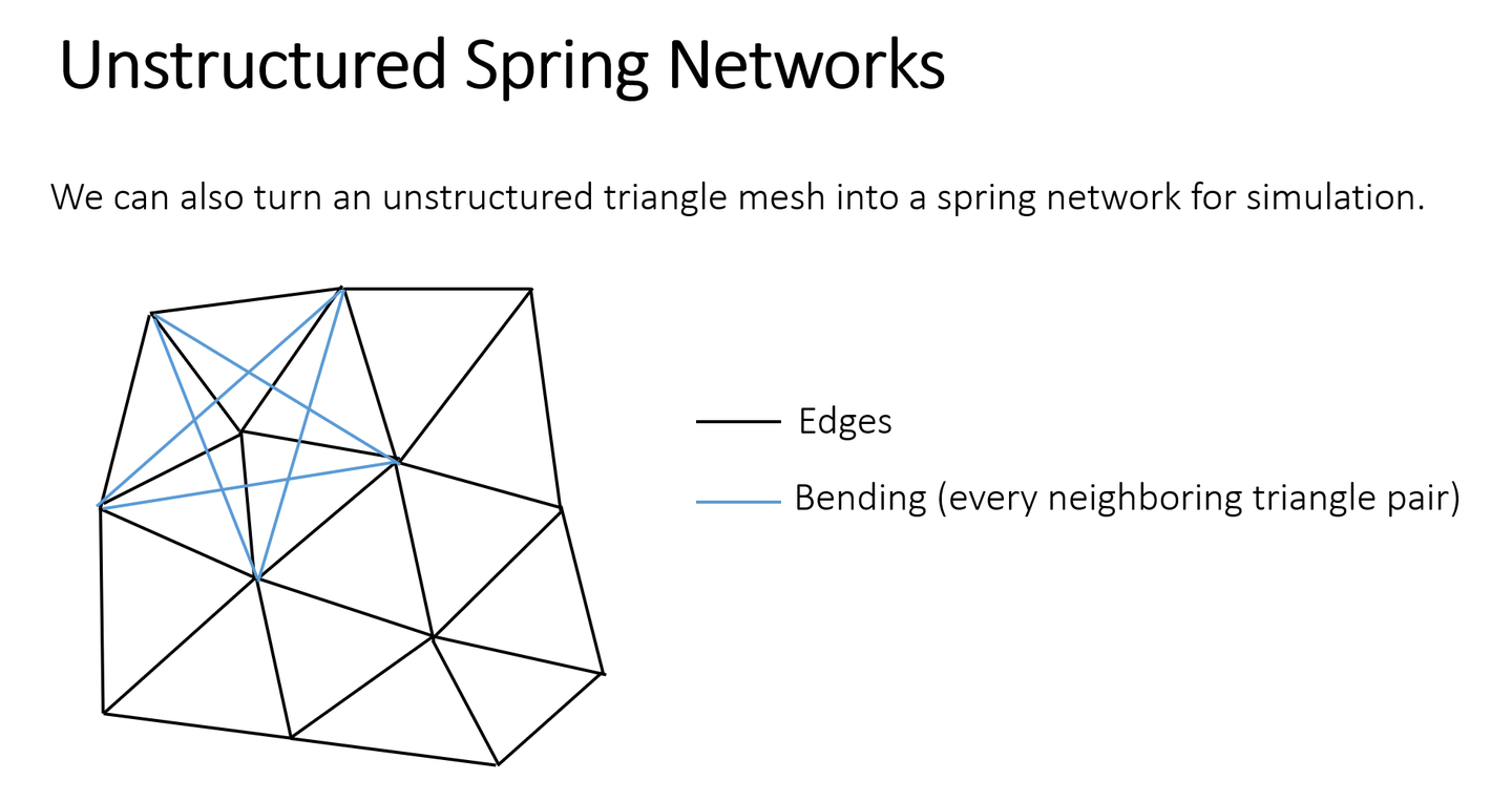
在三角网格的每个边上都加一根弹簧,然后跨过所有内部边添加弹簧(称任意两个相邻三角形的公共边为内部边,两个相邻三角形组成一个四边形,新添加的弹簧为这个四边形的对角线)来抵抗弯曲
边数组(Triple list)的建立:
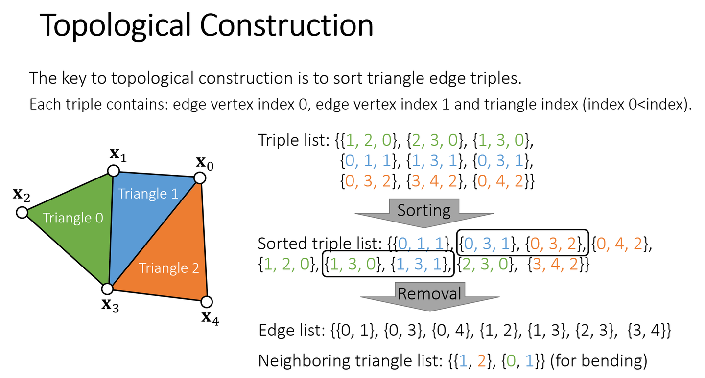
弹簧的建立:
-
对于三角形边上的弹簧,直接遍历 Edge list,依次添加弹簧即可。
-
对于跨过内部边的弹簧,查询内部边所在三角形的剩余两个顶点,把它们连接起来即可。
1.2 Spring Hessian
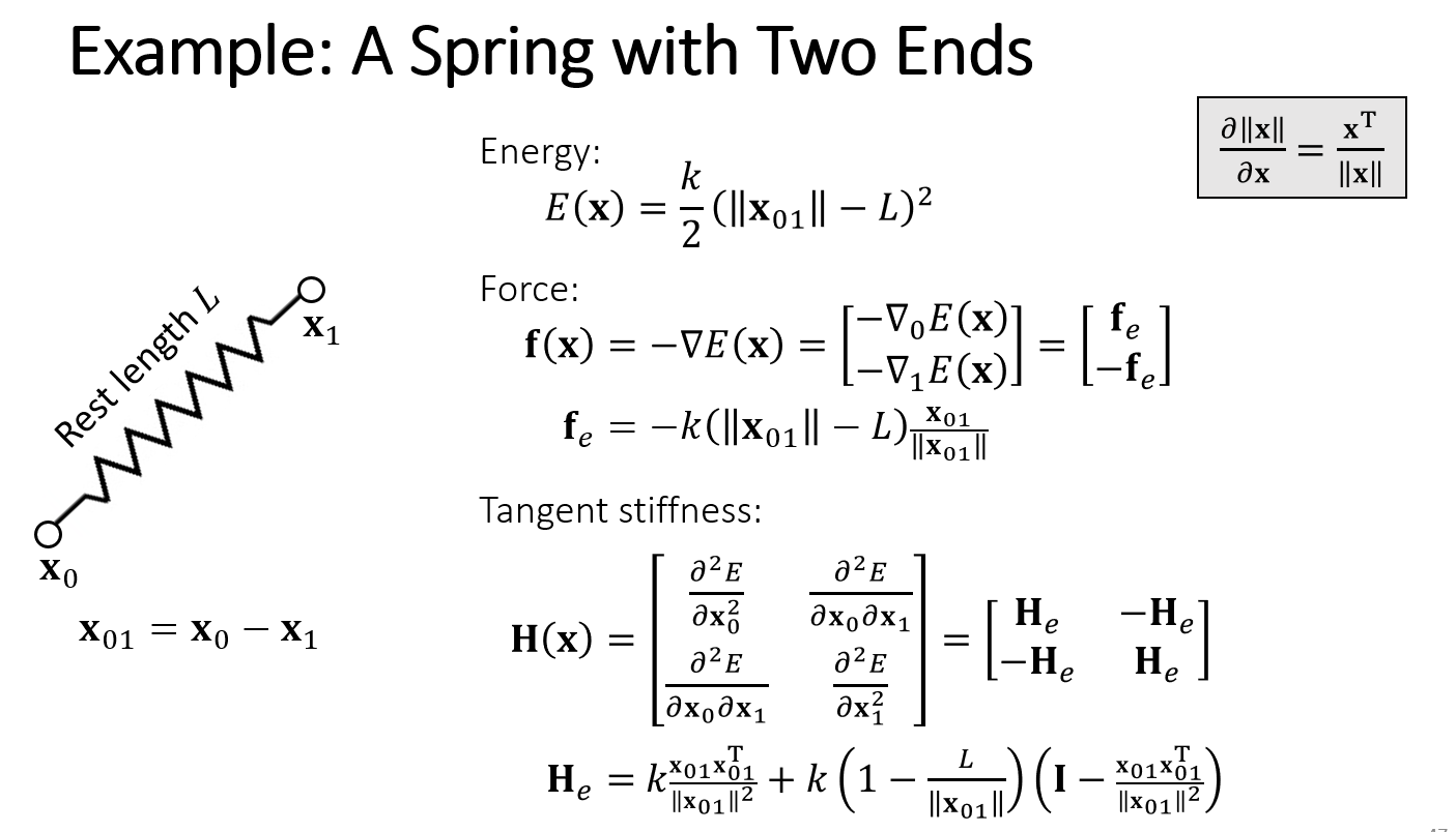
为了计算:
需要先计算Sprint Hessian:
也可以写成:
小矩阵 \(H_e\) 组成大矩阵 \(H\),对角线上的 \(H_e\) 要带上负号
2. Simulation by Newton's Method
其中:
where:
\[\bar x=x^t+\Delta tv^t \]
则
and
where:
- \(H(x^{(k)})\) 就是弹簧系统 \(E(x)\) 的Hessian,
- 弹簧拉伸时,\(H(x)\)一定是SPD,\(\frac{\part^2 F(x^{k})}{\part x^2}\) 一定是SPD,\(F(x)\) 只有一个最小值,牛顿法收敛到唯一的解
- 弹簧压缩时,\(H(x)\)可能不是SPD,\(\frac{\part^2 F(x^{k})}{\part x^2}\) 可能不是SPD
Algorithm:
-
Initialize
-
For \(k=0,...,K\)
-
Solve
\[\left(\frac1{\Delta t^2}M+H(x^{(k)})\right)\Delta x=-\frac1{\Delta t^2}M(x^{(k)}-x^{[0]}-\Delta tv^{[0]})+f(x^{(k)}) \] -
\(x^{(k+1)}\leftarrow x^{(k)}+\Delta x\)
-
-
\(x^{[1]}=x^{(k+1)}\)
-
\(v^{[1]}\leftarrow(x^{[1]}-x^{[0]})/\Delta t\)
where:
- \(x^{[0]}\): 上一帧位置
- \(x^{[1]}\): 这一帧位置
- \(x^{(k)}\), \(x^{(k+1)}\): 上一次/这一次迭代的位置
large step in cloths simulation中的方法:[游戏物理探秘]理解Large Steps in Cloth Simulation - 知乎
-
通过backward Euler的推导,得出:
\[(I-hM^{-1}\frac{\part f}{\part v}-h^2M^{-1}\frac{\part f}{\part x})\Delta v=hM^{-1}(f_0+h\frac{\part f}{\part x}v_0) \] -
解上面的线性系统 \(Ax=b\).
3. 主流模拟方法
3.1 基于物理的模拟
-
Mass-spring system
-
Stretching
-
Bending Issue
- Dihedral angle model
-
Locking Issue
- 本质上,由于自由度缺失,Bending和Stretching不独立
-
Stiffness Issue
-
问题:当stifness大的时候
-
显式积分不稳定,需要减小time step
-
隐式积分ill-condition,需要增加迭代次数
-
要解决这些问题,计算量会增大
-
-
-
-
3.2 非物理的模拟
要满足约束:
$L $是弹簧的原长
投影的思路:使用投影函数,将不满足约束的顶点投影到约束内
投影的方式:Gauss-Seidel,Jacobi
-
Position Based Dynamic:弹性由迭代数量,网格精度体现(顶点多,迭代数量多,则布料会显得更有弹性)
-
过程:
- 先让粒子自由运动
- 投影修改粒子的位置,使粒子满足约束
-
投影的方式:
-
Jacobi迭代
-
GS迭代
-
-
优点:GPU并行
-
缺点
- 没有物理含义
- 顶点多的时候解算很慢,收敛慢
- 迭代过多会导致Locking Issue
解决方案,构建不同分辨率的布料,解算低分辨率的,然后将结果传到高分辨率网格
-
-
Strain Limiting(形变约束)
-
过程:
- 先进行模拟
- 投影修改粒子的位置(相当于纠错),使粒子满足约束(把约束放宽)
-
Spring Strain Limiting(一维的Strain Limiting)
-
\[\sigma^{min}<\phi(x)<\sigma^{max} \]
-
或者写成
-
\[\sigma^{min}<\frac1L||x_i-x_j||<\sigma^{max} \]
-
(当 \(σ=1\) 的时候,就是PBD)
-
-
Triangle Area Limiting
- 当三角的面积超出了约束范围时,直接对三角形进行缩放使面积满足约束。
-
-
Projective Dynamic
-
过程:
-
先让粒子自由运动
-
投影得到新的粒子位置 ,然后用粒子新旧位置更新能量(和原始mass-spring system的力的公式一样)
\[E(x)=\sum\frac k2(||x_i-x_j||-L_e)^2 \] -
然后依然使用隐式积分
-
-
使用Projective Dynamic,能量的Hessian更简单(常数矩阵)
\[f=\nabla E=-k\sum(||x_i-x_j||-L_e)\frac{x_i-x_j}{||x_i-x_j||} \] -
优缺点:
- 有物理意义
- GPU上运行慢
- 迭代一开始收敛快,之后收敛慢
-
-
Constrained Dynamic
- 在隐式积分中引入了对偶变量便于模拟劲度 k 较大的情况
4. Issue
4.1 Locking Issue
Locking Issue: 当Stiffness大时,布料拉不动,也不能弯曲。(比如纸:拉不动,但能弯曲)
解决方法:
- 减小弹簧压缩时的弹性系数
- 使弹簧可以在一定范围内自由移动,超出范围才开始计算弹力
5. Collision Handling
《GPU Gems 3》Chapter 32
3.1 Collision Culling
Spatial Partitioning/Spatial Hashing(对空间划分)
- Morton code:https://www.bilibili.com/video/BV12Q4y1S73g?p=9&vd_source=10edfdf73ab80a5b21d82f049d07a937&t=1947.3
- 使划分后的格子,在内存上访问连续
- GPU friendly,易于实现
- 物体运动后,需要重新计算(计算消耗高)
BVH(对物体划分)
- self-colision的处理
- 不易于实现,Not GPU friendly(GPU不易存储树)
- 更新树时,不需要更新树的结构,只需要更新bounding volumes
3.2 Collision Test
Discrete Collision Detection(DCD)
- Edge-triangle pairs
- 只检测某状态是否相交,不能检测穿透
Continuous Collision Detection
-
Vertex-triangle pairs
- vertex和triangle构成的四面体,面积为0
- 每个顶点位置都是 \(t\) 的一次函数,解一元三次方程(用二分法,3个顶点所以是三次方程)判断四面体面积为0时(即vertex和triangle在同一平面),vertex是否在triangle内
-
Edge-edge pairs
-
难写,性能消耗大,游戏GPU以单浮点精度为主
碰撞处理:
-
Interior point method
- 每一次运动后都满足碰撞约束
- 慢(需要处理所有vertex)
- Always succeed
-
Impact zone optimization
- 逃出约束之后,再慢慢纠正
- 快(只需要处理碰撞的vertex)
- May not succeed
课后阅读论文:Robust Treatment of Collisions, Contact and Friction for Cloth Animation(TOG SIGGRAPH 2002)

 浙公网安备 33010602011771号