（模拟）迭代方法与Multigrid

首先，老规矩：

未经允许禁止转载(防止某些人乱转，转着转着就到蛮牛之类的地方去了)

B站:Heskey0

---

一，Iterative Method

《Iterative Method for Sparse Linear System》

Pre. 线性代数的本质

行列式：面积的缩放倍数

特征向量：矩阵变换后，某方向的向量不发生旋转（仅发生缩放，缩放倍数为特征值）

Gaussian Elimination：高斯消元，可理解为矩阵的行变换。

Matrix Polynomial: \(p(A)=a_0I+a_1A+a_2A^2+...+a_nA^n\)

Frobenius norm (F-范数)

是一种矩阵范数

\[||A||_F=(\sum^m_{j=1}\sum^n_{i=1}|a_{ij}^2|)^{1/2} \]

linear span (线性生成空间)：向量集 S 的生成空间也可定义为 S 中元素的所有有限线性组合组成的集合

\[span(S)=span(v_1,...,v_r)=\{\lambda_1+...+\lambda_rv_r\} \]

M矩阵：实方阵A=[aij]的非对角元均非正(即aij≤0,i≠j),且其所有主子式均为正,则称其为闵可夫斯基矩阵,简称M矩阵

Cholesky factorization：Cholesky factorization）-CSDN博客_乔里斯基分解法

若 \(A\) 是SPD的 \(n\times n\)矩阵，则可以分解为

\[A=LL^T \]

其中 \(L\) 为下三角矩阵

Chapter 1. Background in Linear Algebra

1.2 Square Matrices and Eigenvalues

spectral radius：The maximum modulus of the eigenvalues

\[\rho(A)=\max|\lambda| \]

• 当B的谱半径小于1时这个系统会收敛但是当谱半径接近1时收敛速度很慢。

• The spectral radius is considered to be an asymptotic measure of convergence because it predicts the worst-case error reduction over many iterations

1.3 Types of Matrices

nonsingular matrix：非奇异矩阵是行列式不为 0 的矩阵，也就是可逆矩阵

1.5 Matrix Norm

【定义】

可以由向量范数诱导出矩阵范数：

\[||A||_{pq}=\max_{x\in C^m,x\ne0}\frac{||Ax||_p}{||x||_1} \]

其中 \(p,q=1,2,\infin\)

当 \(q=p\) 时，称为 p-norm

【性质】

• \(||AB||_p\le ||A||_p||B||_p\)
• 谱半径不大于矩阵范数：\(\rho(A)\le||A||\)

\[||A||_1=\max_{j=1,...,m}\sum^n_{i=1}|a_{ij}|\\ ||A||_\infin=\max_{i=1,...,n}\sum^m_{j=1}|a_{ij}| \]

1.6 Subspaces, Range, and Kernel

vector subspace： 向量空间V的非空子集W，满足W对于V的加法和数量乘法具有封闭性

两个重要的 vector subspace：range，kernel

range：像空间

\[Ran(A)=\{Ax|x\in\C^m\} \]

\(A\) is a matrix of \(\C^{n\times m}\)

kernel/null space：零空间

\[Ker(A)=\{x\in\C^m|Ax=0\} \]

1.7 Orthogonal Vectors and Subspaces

Gram-Schmidt： Gram Schmidt Process 把一组普普通通的basis转换为相互正交的basis

QR decomposition：QR分解 将矩阵 \(A=QR\) 分解成正交矩阵 \(Q\) 和上三角矩阵 \(R\)

Householder：Householder变换 是一种能将n维向量x变换到任一n维向量y的正交变换

1.8 Canonical Forms of Matrices

Two matrices \(A\) and \(B\) is said to be similar if there is a nonsingular matrix \(X\) such that

\[A=XBX^{-1} \]

The mapping \(B\rightarrow A\) is called a similarity transformation

1.9 Normal and Hermitian Matrices

Normal Matrix：正规矩阵，满足 \(A^HA=AA^H\)

Hermitian Matrix：复共轭对称矩阵（矩阵中第i行第j列是第j行第i列的元素的共轭）

\(a_{i,j}=\bar{a}_{j,i}\)记作：\(A=A^H\)

1.11 Positive-Definite Matrices

线性代数——二次型 - 知乎

正定矩阵

positive define matrix：\(x^TMx>0\)，则称M为正定矩阵，\(f(x)=x^TMx\) 为正定二次型

定理：

（1）正定矩阵可逆

判定：

（1）A是正定矩阵；

（2）A的一切顺序主子式均为正；

（3）A的一切主子式均为正；

（4）A的特征值均为正；

（5）存在实可逆矩阵C，使A=C′C；

（6）存在秩为n的m×n实矩阵B，使A=B′B；

（7）存在主对角线元素全为正的实三角矩阵R，使A=R′R

1.12 Projection Operators

projection：a projector \(P\) is any linear mapping from \(C^n\) to itself which is idempotent.

Orthogonal projection：正交投影，是指像空间U和零空间W相互正交子空间的投影

projection operator：投影算子是赋范线性空间 \(X\) 上具有幂等性的有界线性算子，设 \(P\) 是 \(X\) 上的有界线性算子，如果 \(P^2=P\)，则称 \(P\) 为投影算子。

define: \(Ran(P)=M\) and \(Null(P)=S\).

In fact, an arbitrary projector \(P\) can be entirely determined by two subspaces:

1. The range \(M\) of \(P\)
2. its null space \(S\) which is also the range of \(I-P\), i.e. \(S=Null(P)=Ran(I-P)\)

For any \(x\), the vector \(Px\) satisfies the conditions,

\[Px\in M\\ x-Px\in S \]

The linear mapping \(P\) is said to project \(x\) onto \(M\) and along or parallel to the subspace \(S\).

define: \(L=S^\perp\) and \(u=Px\) , then

\[u\in M\\ x-u\perp L \]

These equations define a projector \(P\) onto \(M\) and orthogonal to the subspace \(L\).

Orthogonal Projector: L is equal to M

Theorem:

• Let \(P\) be the orthogonal projector onto a subspace \(M\). Then for any vector \(x\) in \(C^n\):
  \[\min_{y\in M}||x-y||_2=||x-Px||_2 \]

1.13 Basic Concepts in Linear Systems

1.13.1 Existence of a Solution

\[Ax=b \]

解的情况：

• Case 1：\(A\) is nonsingular (可逆)

  • unique solution given by: \(x=A^{-1}b\)

• Case 2：\(A\) is singular, and \(b\in Ran(A)\)

  • infinitely many solutions

• Case 3：\(A\) is singular, and \(b\notin Ran(A)\)

  • no solutions

1.13.2 Perturbation Analysis

condition number：

\[\kappa(A)=||A||\,||A^{-1}|| \]

SPD(Symmetric Positive Define)矩阵的condition number：

最大特征值除以最小特征值

\[\kappa(A)=\lambda_{max}/\lambda_{min} \]

In addition, small eigenvalues do not always give a good indication of poor conditioning. Indeed, a matrix can have all its eigenvalues equal to one yet be poorly conditioned.

• condition number是线性方程组Ax=b的解对b中的误差或不确定度的敏感性的度量，condition number 越小，收敛越快

特征值的小，不代表线性系统的poor conditioning

Chapter 2. Discretization of PDEs

​ PDE is the biggest source of sparse matrix problems. The typical way to solve such equations is to discretize them, i.e. to approximate them by equations that involve a finite number of unknowns.

本章介绍PDE discretize的三种方法：

• The simplest method uses finite difference approximations for the partial differential operators.
• The Finite Element Method replaces the original function by a function which has some degree of smoothness over the global domain, but which is piecewise polynomial on simple cells, such as small triangles or rectangles.
• 在上两种方法之间，there are a few conservative schemes called Finite Volume Methods, which attempt to emulate continuous conservation laws of physics.

2.1 Partial Differential Equations

2.1.1 Elliptic Operators

Poisson's equation：工程界最常见的一种PDE

\[\frac{\part^2u}{\part x_1^2}+\frac{\part^2u}{\part x_2^2}=f \]

for \(x = (x_1,x_2)\) a vector

Domain \(\Omega\)：Poisson's equation中，\(x\) 所属的bounded open domain

\(\vec n\)：unit vector, normal to the boundary \(\Gamma\) and directed outwards.

Boundary condition：

• Dirichlet condition：\(u(x)=\phi(x)\)
• Neumann condition：\(\frac{\partial u}{\partial \vec n}=0\) ，是Cauchy condition的特殊情况（\(\gamma=\alpha=0\)）
• Cauchy condition：\(\frac{\partial u}{\partial \vec n}+\alpha(x)u(x)=\gamma(x)\)

Laplace equation

\[\Delta u=0 \]

its solutions are called harmonic function

Laplacean operator

\[\Delta=\frac{\part^2}{\part x_1^2}+\frac{\part^2}{\part x_2^2} \]

2.1.2 The Convection Diffusion Equation

Many physical problems involve a combination of “diffusion” and “convection” phenomena. Such phenomena are modeled by the convection-diffusion equation：

\[\frac{\part u}{\part t}+b_1\frac{\part u}{\part x_1}+b_2\frac{\part u}{\part x_2}=\nabla\cdot (a\nabla)u+f \]

2.2 Finite Difference Methods

The finite difference method is based on local approximations of the partial derivatives in a Partial Differential Equation, which are derived by low order Taylor series expansions.

2.2.1 Basic Approximation

• Forward difference，一阶泰勒展开

  \[\frac{\part q}{\part x}\approx\frac{q_{i+1}-q_i}{\Delta x}=\frac{u(x+h)-u(x)}{h} \]

• backward difference

• central difference(unbiased, 精度高)，两个二阶泰勒展开

  \[\frac{\part q}{\part x}\approx\frac{q_{i+1}-q_{i-1}}{2\Delta x} \]

  改进：(staggered grid)

  \[\frac{\part q}{\part x}\approx\frac{q_{i+1/2}-q_{i-1/2}}{\Delta x} \]

2.2.2 Difference Schemes for the Laplacean Operator

\[\begin{aligned} \Delta u(x)\approx &\frac{u(x_1+h,x_2)+u(x_1-h,x_2)-2u(x_1,x_2)}{h_1^2}\\&\frac{u(x_1+h,x_2)+u(x_1-h,x_2)-2u(x_1,x_2)}{h_2^2} \end{aligned} \]

当 \(h_1=h_2时\)：

\[\begin{aligned} \Delta u(x)\approx &\frac1{h^2}[u(x_1+h,x_2)+u(x_1-h,x_2)\\&+u(x_1,x_2+h)+u(x_1,x_2-h)\\&-4u(x_1,x_2)] \end{aligned} \]

Mesh size：网格的大小 \(h,h_1,h_2\)

2.2.3 Finite Differences for 1-D Problems

Consider the 1-D equation：

\[-u^{\prime\prime}(x)=f(x)\quad for\,\,\,x\in(0,1)\\ u(0)=u(1)=0 \]

The interval \([0,1]\) can be discretized uniformly by taking the \(n+2\) points

\[x_i=i\times h,\quad i=0,...,n+1 \]

where \(h=1/(n+1)\)

Because of the Dirichlet boundary conditions, the values \(u(x_0)\) and \(u(x_{n+1})\) are known. At every other point, an approximation \(u_i\) is sought for the exact solution \(u(x_i)\)

If the centered difference approximation is used, then:

\[\frac{-u_{i-1}+2u_i-u_{i+1}}{h^2}=f_i \]

in which \(f_i=f(x_i)\) .

for \(i=1\) and \(i=n\)，\(u_0=u_{n+1}=0\) in this case. Thus, for \(n=6\)，the linear system obtained is of the form

\[Ax=f \]

where

\[A=\frac1{h^2} \left( \begin{array}{1} 2&-1&&&&\\ -1&2&-1&&&\\ &-1&2&-1&&\\ &&-1&2&-1&\\ &&&-1&2&-1\\ &&&&-1&2 \end{array} \right) \]

\(n\) 越大，则grid越密，且 \(A\) 越大，解向量 \(x\) 的维度越大

2.2.5 Finite Differences for 2-D Problems

Consider the 2-D equation：

\[\begin{aligned} -\left(\frac{\part^2 u}{\part x_1^2}+\frac{\part^2 u}{\part x_2^2}\right)=f\quad &in\,\, \Omega\\ u=0\quad &on\,\, \Gamma \end{aligned} \]

where \(\Omega\) is now the rectangle \((0,l_1)\times(0,l_2)\) and \(\Gamma\) its boundary

类似2.2.3节，可以得到一个二维的网格（网格的粒度由discretize所用的点的数量决定），由于Dirichlet Boundary condition（边界点的值已知为0），所以只考虑内部的点（忽略网格边界的点）

the linear system obtained is of the form (\(7\times5\) finite difference)

\[Ax=b \]

\[A=\frac1{h^2}\left( \begin{array}{1} B&-I&\\ -I&B&-I\\ &-I&B \end{array} \right),x=\pmatrix{u_{11}\\u_{12}\\...\\u_{15}\\u_{21}\\...\\u_{25}\\u_{31}\\...\\u_{35}} \]

with

\[B=\left( \begin{array}{1} 4&-1&&\\ -1&4&-1&\\ &-1&4&-1&\\ &&-1&4&-1\\ &&&-1&4 \end{array} \right) \]

grid mesh and matrix：

个人理解：矩阵分九个方格 （\(i\times j=3\times3\)）

• 每 \(i\) 行中，第 \(j\) 个方格代表grid mesh的第 \(j\) 行 (grid mesh有3行，所以矩阵每一行有3个方格)
• 第 \(i\) 行代表标号为 \(i\) 的grid point
• 矩阵中，有一些 \(-1\) 的元素缺失，是因为点在grid mesh中处于边界条件

不规则网格：

通过对规则网格的理解，来看上图中的不规则网格，思考下列过程（仅限于该案例）：

• 向量 \(u_1,u_2,...,u_{48}\) 按照grid mesh中的标号进行排序
• 矩阵的第一行与向量的乘积：\(4\times u_1-u_2-u_4\)
• 按照grid mesh中的vertex based domain decomposition
  • \(u_1,...u_{16}\) 处于一个domain，对应到矩阵 \(A\) 的1-16行
  • domain decomposition就相当于矩阵 \(A\) 的按行分割
  • 若不考虑subdomain之间的boundary condition（或者说inteface），则 \(A\) 可以沿对角线方向分割成多个矩阵（如下图）
    

2.3 Finite Element Method

​ FEM belongs to the family of Galerkin methods.

Typical steps:

1. Convert strong-form PDEs to weak forms, using a test function \(w\).
2. Integrate by parts to redistribute gradient operators.
3. Use the divergence theorem to simplify equations and enforce Neumann boundary conditions (BCs).
4. Discretization (build the stiffness matrix and right-hand side).
5. Solve the (discrete) linear system.

2.3.1 Notation

Consider the 2-D equation：

\[\begin{aligned} -\left(\frac{\part^2 u}{\part x_1^2}+\frac{\part^2 u}{\part x_2^2}\right)=f\quad &in\,\, \Omega\\ u=0\quad &on\,\, \Gamma \end{aligned} \]

where \(\Omega\) is now the rectangle \((0,l_1)\times(0,l_2)\) and \(\Gamma\) its boundary

The Green's formula：

\[\int_\Omega\nabla v.\nabla u\quad dx=-\int_\Omega v\Delta u\quad dx+\int_\Gamma v\frac{\part u}{\part \vec n}ds \]

where \(v\) is a vector-valued function \(\vec v=\pmatrix{v_1\\v_2}\)

To solve this problem approximately, it is necessary to：

1. take approximations to the unknown function \(u\)
2. translate the equations into a system which can be solved numerically

Let us define:

\[a(u,v)=\int_\Omega\nabla u.\nabla v\, dx=\int_\Omega\left(\frac{\part u}{\part x_1}\frac{\part v}{\part x_1}+\frac{\part u}{\part x_2}\frac{\part v}{\part x_2}\right)\\ (f,v)=\int_\Omega fv\,dx \]

2.3.2 FEM推导

The original domain is approximated by union \(\Omega_h\) of \(m\) triangles \(K_i\),

\[\Omega_h=\bigcup^m_{i=1}K_i \]

Then the finite dimensional space \(V_h\) is defined as the space of all functions which are piecewise linear and continuous on the polygonal region \(Ω_h\), and which vanish on the boundary \(Γ\) :

\[V_h=\{\phi|\phi_{|\Omega_h}\,continuous,\phi_{|\Gamma_h}=0,\phi_{|K_j}linear\,\forall j\} \]

Here, \(\phi_{|X}\) represents the restriction of the function \(\phi\) to the subset X. If \(x_j , j = 1, . . ., n\) are the nodes of the triangulation, then a function \(\phi_j\) in \(V_h\) can be associated with each node \(x_j\) , so that the family of functions \(\phi_j\)’s satisfies the following conditions:

\[\phi_j(x_i)=\delta_{ij}=\left\{ \begin{aligned} 1\quad if\quad x_i=x_j\\ 0\quad if \quad x_i\ne x_j \end{aligned} \right. \]

In addition, the \(\phi_i\)'s form a basis of the space \(V_h\). Each function of \(V_h\) can be expressed as:

\[\phi(x)=\sum^n_{i=1}\xi_i\phi_i(x) \]

The finite element approximation consists of writing the Galerkin condition for functions in \(V_h\). This defines the problem:

\[{Find}\quad u\in V_h\quad such \,\,that\quad a(u,v)=(f,v),\quad \forall v\in V_h \]

Writing the desired solution \(u\) in the basis \(\{\phi_i\}\) as:

\[u=\sum^n_{j=1}\xi_j\phi_j(x) \]

带入上式 \(a(u,v)=(f, v)\)，得到：

\[\sum^n_{j=1}\alpha_{ij}\xi_j=\beta_i \]

where:

\[\alpha_{ij}=a(\phi_i,\phi_j),\quad \beta_i=(f,\phi_i) \]

The above equations form a linear system of equations \(Ax=b\), in which the coefficients of \(A\) are the \(a_{ij}\)'s; those of \(b\) are the \(\beta_j\)'s. In addition, \(A\) is a SPD matrix. (\(\int_\Omega\nabla\phi_i.\nabla\phi_j\,dx=\int_\Omega\nabla\phi_j.\nabla\phi_i\,dx\) ).

​ In practice, the matrix is built by summing up the contributions of all triangles by applying the formula:

\[a(\phi_i,\phi_j)=\sum_Ka_K(\phi_i,\phi_j)\\ a_K(\phi_i,\phi_j)=\int_K\nabla\phi_i\nabla\phi_j\,dx \]

Thus, a triangle contributes nonzero values to its three vertices from the above formula. The \(3\times3\) matrix

\[A_K=\pmatrix{ a_K(\phi_i,\phi_i)&a_K(\phi_i,\phi_j)&a_K(\phi_i,\phi_k)\\ a_K(\phi_j,\phi_i)&a_K(\phi_j,\phi_j)&a_K(\phi_j,\phi_k)\\ a_K(\phi_k,\phi_i)&a_K(\phi_k,\phi_j)&a_K(\phi_k,\phi_k) } \]

associated with the triangle \(K(i,j,k)\) with vertices \(i,j,k\) is called an element stiffness matrix. In order to form the matrix \(A\), it is necessary to sum up all the contributions \(a_K(\phi_k,\phi_m)\) to the position \(k, m\) of the matrix. This process is called an assembly process. In the assembly, the matrix is computed as:

\[A=\sum^{nel}_{e-1}A^{[e]} \]

2.3.3 FEM的直观理解

The four elements are numbered from bottom to top as indicated by the labels located at their centers. There are six nodes in this mesh and their labeling is indicated in the circled numbers. The four matrices \(A^{[e]}\) associated with these elements are shown in Figure 2.9(下图). Thus, the first element will contribute to the nodes 1, 2, 3, the second to nodes 2, 3, 5, the third to nodes 2, 4, 5, and the fourth to nodes 4, 5, 6:

2.4 Mesh Generation and Refinement

2.5 Finite Volume Method

Chapter 3. Sparse Matrix

Standard discretization of PDEs typically lead to large and sparse matrices. Some sparse matrix techniques begin with the idea that the zero elements need not be stored. This chapter gives an overview of sparse matrices, their properties, their representations, and the data structures used to store them.

3.1 Introduction

two broad types of matrices: structured and unstructured

Python稀疏矩阵详解 - 知乎 (zhihu.com)

3.2 稀疏矩阵的存储形式

coo:

coo_matrix的优点：

• 有利于稀疏格式之间的快速转换（tobsr()、tocsr()、to_csc()、to_dia()、to_dok()、to_lil()）
• 允许又重复项（格式转换的时候自动相加）
• 能与CSR / CSC格式的快速转换

coo_matrix的缺点：

• 不能直接进行算术运算

csr：（compressed sparse row）

csr_matrix的优点：

• 高效的算术运算CSR + CSR，CSR * CSR等
• 高效的行切片
• 快速矩阵运算

csr_matrix的缺点：

• 列切片操作比较慢（考虑csc_matrix）
• 稀疏结构的转换比较慢（考虑lil_matrix或doc_matrix）

csc：（compressed sparse column）

优缺点和csr_matrix一致

LiL：（List of Lists format）

LIL format优点

• 支持灵活的切片操作「行切片操作效率高，列切片效率低」
• 稀疏矩阵格式之间的转化很高效（tobsr()、tocsr()、to_csc()、to_dia()、to_dok()、to_lil()）

LIL format缺点

• 加法操作效率低 (consider CSR or CSC)
• 列切片效率低(consider CSC)
• 矩阵乘法效率低 (consider CSR or CSC)

dok：（Dictionary Of Keys based sparse matrix）

是一种类似于coo matrix但又基于字典的稀疏矩阵存储方式，key由非零元素的的坐标值tuple(row, column)组成，value则代表数据值。dok matrix非常适合于增量构建稀疏矩阵，并一旦构建，就可以快速地转换为coo_matrix。

dia：（Sparse matrix with DIAgonal storage）

bsr：（Block Sparse Row matrix）

bsr_matrix可用于算术运算：支持加法，减法，乘法，除法和矩阵幂。对于许多稀疏算术运算，BSR比CSR和CSC更有效

Chapter 4. Basic Iterative Methods

4.1 Point Relaxation Scheme

solving \(Ax=b\)

We split matrix \(A\) in the form

\[A=D+L+U \]

where

• \(D\) the diagonal of \(A\)
• \(L\) and \(U\) the lower and upper triangular parts of \(A\)

Jacobi method

\[x^{(k+1)}=D^{-1}[b-(L+U)x^{(k)}] \]

Damped Jacobi （weighted Jacobi）建议 \(\omega=\frac23\)

\[x^{(k+1)}=\omega D^{-1}[b-(L+U)x^{(k)}]+(1-\omega)x^{(k)} \]

Gauss-Seidel

\[x^{(k+1)}=(D+L)^{-1}(b-Ux^{(k)}) \]

\[x^{(k+1)}_i=\frac1{a_{ii}}\left(b_i-\sum^{i-1}_{j=1}a_{ij}x_j^{(k+1)}-\sum^n_{j=i+1}a_{ij}x^{(k)}_j\right) \]

依次算出 \(x^{(k+1)}\) 的component

Successive Over Relaxation （SOR，超松弛）

\[x^{(k+1)}=(D+\omega L)^{-1}(\omega b-[\omega U+(\omega-1)D]x^{(k)}) \]

\[x^{(k+1)}_i=(1-\omega)x^{(k)}_i+\frac\omega{a_{ii}}\left(b_i-\sum^{i-1}_{j=1}a_{ij}x_j^{(k+1)}-\sum^n_{j=i+1}a_{ij}x^{(k)}_j\right) \]

当 \(\omega=1\) 时，

Damped Jacobi == Jacobi

SOR == Gauss-Seidel

• 当B的谱半径小于1时这个系统会收敛但是当谱半径接近1时收敛速度很慢。

• SOR就是为了减少谱半径所施加的一些小代数技巧。

for Gauss–Seidel, the order of updating is significant. Instead of sweeping through the components in ascending order, we could sweep through the components in descending order.

symmetric Gauss-Seidel：alternate between ascending and descending orders

red-black Gauss-Seidel：ordering that results by coloring the gridpoints red and black in a checkerboard pattern. All red(even) points are updated before the black(odd) points.

4.2 Block Relaxation Schemes

​ Block Relaxation Schemes update a whole set of components at each time, typically a subvector of the solution vector, instead of only one component.

\[A=\pmatrix{ A_{11}&A_{12}&A_{13}&...&A_{1p}\\ A_{21}&A_{22}&A_{23}&...&A_{2p}\\ A_{31}&A_{32}&A_{33}&...&A_{3p}\\ &...&&...&\\ A_{p1}&A_{p2}&A_{p3}&...&A_{pp} }, x=\pmatrix{ \xi_1\\\xi_2\\\xi_3\\...\\\xi_4} ,b=\pmatrix{ \beta_1\\\beta_2\\\beta_3\\...\\\beta_p } \]

in which the partitionings of \(b\) and \(x\) into subvectors \(\beta_i\) and \(\xi_i\) are identical and compatible with the partitioning of \(A\).

\[(Ax)_i=\sum^p_{j=1}A_{ij}\xi_j \]

Consider:

• a set-decomposition \(S=\{1,2,...,n\}\)
• \(p\) 个 subsets \(S_1,...,S_p\) with \(\cup S_i=S\)
• Denote by \(n_i\) the size of \(S_i\) and define \(S_i=\{m_i(1),m_i(2),...,m_i(n_i)\}\)
• the \(n\times n_i\) matrix \(V_i=[e_{m_i(1)},e_{m_i(2)},...,e_{m_i(n_i)}]\)
  • where each \(e_j\) is the \(j\)-th column of the \(n\times n\) identity matrix.

Then Let:

• \(V_i\) be the \(n\times n_i\) matrix

  \[V_i=[e_{m_i(1)},e_{m_i(2)},...,e_{m_i(n_i)}] \]

• \[W_i=[\eta_{m_i(1)}e_{m_i(1)},\eta_{m_i(2)}e_{m_i(2)},...,\eta_{m_i(n_i)}e_{m_i(n_i)}] \]

where each \(e_j\) is the column of the \(n\times n\) identity matrix, and \(\eta_{m_i(j)}\) represents a weight factor chosen so that:

\[W^T_{i}V_i=I \]

• When there is no overlap, then define \(\eta_{m_i(j)}=1\)

Then: (\(W^T_i\) 和 \(V_j\) 的作用就是取出 \(A\) 中的某一部分)

• \(A_{ij}=W^T_iAV_j\)
• \(\xi_i=W^T_i x,\quad \beta_i=W^T_ib\)
• \(x=\sum V_i\xi_i\)

4.2.1 Introduction

​ With finite diference, it is standard to block the variables and the matrix by partitioning along whole lines of the mesh.

grid mesh:

matrix:

block techniques can be defined in more general terms:

• by using blocks that allow us to update arbitrary groups of components
• by allowing the blocks to overlap.

our partition has been based on an actual set-partition of the variable set \(S=\{1,2,...,n\}\) into subsets \(S_1,S_2,...,S_p\), with the condition that two distinct subsets are disjoint. More generally, a set-decomposition of \(S\) removes the constraint of disjointness.

4.2.2 Algorithm

Block Jacobi method:

\[A_{ii}x_i^{(k+1)}=b_i-\sum^p_{j=1,j\ne i}A_{ij}x_j^{(k)}\quad,i=1,...,p \]

Block Jacobi Iteration:

1. For \(k=0,1,...,\) until convergence Do:
   1. For \(i=1,2,...,p\) Do:
      1. Solve \(A_{ii}\delta_i=W^T_i(b-Ax_k)\)
      2. Set \(x_{k+1}=x_k+V_i\delta_i\)
   2. EndDo
2. EndDo

Block Gauss-Seidel Iteration：

1. Until convergence Do:
   1. For \(i=1,2,...,p\) Do:
      1. Solve \(A_{ii}\delta_i=W^T_i(b-Ax)\)
      2. Set \(x=x+V_i\delta_i\)
   2. EndDo
2. EndDo

Block Jacobi/GS的 main loop (lines 2 to 5) represents an orthogonal projection process over \(K_i=span\{V_i\}\)

Chapter 5. Projection Methods

Projection method就是：

1. 在search subspace \(K\) 中选取一个 \(x\)，将其投影到 \(Ran(A)\)（即矩阵 \(A\) 的子空间range），得到 \(Ax\).
2. 目标解 \(u\) 投影到 \(Ran(A)\)，得到 \(Au=b\).
3. 此时 \(Ax\) 与 \(Au=b\) 都在 \(Ran(A)\) 中，且 \(b-Ax\perp L\)
4. 不断跳转到 step1，minimize the residual

\(K\) 就是自由度的体现，\(L\) 就是约束的体现.

A projection process represents a canonical way for extracting an approximation to the solution of a linear system from a subspace.

​ A projection technique onto the subspace \(K\)(search subspace) and orthogonal to \(L\)(subspace of constraints) is a process which finds an approximate solution \(\tilde x\) to \(Ax=b\) by imposing the conditions that \(\tilde x\) belong to \(K\) and that the new residual vector be orthogonal to \(L\):

\[Find\quad \tilde x\in x_0+K,\quad such\,\,\, that\quad b-A\tilde x\perp L \]

即：

\[\tilde x=x_0+\delta,\quad \delta\in K\\ (r_0-A\delta,w)=0,\quad \forall w\in L \]

affine subspace：\(x_0+K\)

Petrov-Galerkin conditions：\(b-Ax\perp L\)

when \(L=K\)，the Petrov-Galerkin conditions are called the Galerkin conditions

\(x_0\)：initial guess

orthogonal projection：\(L=K\)

oblique projection：\(L\ne K\)

5.1 Prototype Projection Method

5.1.1 General Projection Methods

​ In fact, virtually all of the basic iterative techniques seen in the previoud chapter can be considered projection techniques. Whenever an approximation is defined via \(m\) degrees of freedom (subspace \(K\)) and \(m\) constraints (subspace \(L\)), a projection process results.

5.1.2 Matrix Representation

Let \(V=[v_1,...,v_m]\), an \(n\times m\) matrix whose column-vectors form a basis of \(K\) and, \(W=[w_1,...,w_m]\), an \(n\times m\) matrix whose column-vectors form a basis of \(L\).

Prototype Projection Method：

1. Until convergence, Do:
   1. Select a pair of subspace \(K\) and \(L\)
   2. Choose bases \(V=[v_1,...,v_m]\) and \(W=[w_1,...w_m]\) for \(K\) and \(L\)
   3. \(r=b-Ax\)
   4. \(y=(W^TAV)^{-1}W^Tr\)
   5. \(x=x+Vy\)
2. EndDo

5.2 General Theory

​ This section gives some general theoretical results without being specific about the subspaces \(K\) and \(L\) which are used. The goal is to learn about the quality of the approximation obtained from a general projection process. Two main tools are used for this.

• The first is to exploit optimality properties of projection methods. These properties are induced from those properties of projectors seen in Section 1.12.4 of Chapter 1.
• The second tool consists of interpreting the projected problem with the help of projection operators in an attempt to extract residual bounds.

5.3 One-Dimensional Projection Processes

\[K=spac\{v\}\quad and\quad L=span\{w\} \]

where \(v\) and \(w\) are two vectors. In this case, the new approximation takes the form \(x\leftarrow x+\alpha v\) and the Petrov-Galerkin condition \(r-A\delta \perp w\) yields

\[\alpha=\frac{(r,w)}{(Av,w)} \]

Steepest Descent Algorithm：

1. Until convergence, Do:
   1. \(r\leftarrow b-Ax\)
   2. \(\alpha\leftarrow (r,r)/(Ar,r)\)
   3. \(x\leftarrow x+\alpha r\)
2. EndDo

each step minimizes \(f(x)=||x-x_\star||^2_A=(A(x-x_\star),(x=x_\star))\) over all vectors of the form \(x+\alpha d\), where \(d=-\nabla f\)

Minimal Residual Iteration：

1. Until convergence, Do:
   1. \(r\leftarrow b-Ax\)
   2. \(\alpha\leftarrow (Ar,r)/(Ar,Ar)\)
   3. \(x\leftarrow x+\alpha r\)
2. EndDo

each step minimizes \(f(x)=||b-Ax||^2_2\) in the direction \(r\).

Residual Norm Steepest Descent：

1. Compute \(r=b-Ax\)
2. Until convergence, Do:
   1. \(v=A^Tr\)
   2. Compute \(Av\) and \(\alpha=||v||^2_2/||Av||^2_2\)
   3. \(x=x+\alpha v\)
   4. \(r=r-\alpha Av\)
3. EndDo

each step minimizes \(f(x)=||b-Ax||^2_2\) in the direction \(-\nabla f\).

5.4 Additive and Multiplicative Processes

Consider:

• a set-decomposition \(S=\{1,2,...,n\}\)
• \(p\) 个 subsets \(S_1,...,S_p\) with \(\cup S_i=S\)
• Denote by \(n_i\) the size of \(S_i\) and define \(S_i=\{m_i(1),m_i(2),...,m_i(n_i)\}\)
• the \(n\times n_i\) matrix \(V_i=[e_{m_i(1)},e_{m_i(2)},...,e_{m_i(n_i)}]\)
  • where each \(e_j\) is the \(j\)-th column of the \(n\times n\) identity matrix.

Additive Projection Procedure: 累加

1. For \(k=0,1,...\) until convergence, Do:
   1. For \(i=1,2,...,p\) Do:
      1. Solve \(A_iy_i=V^T_i(b-Ax_k)\)
   2. EndDo
   3. Set \(x_{k+1}=x_k+\sum^p_{i=1}V_iy_i\)
2. EndDo

the general block Jacobi iteration combines these modifications, implicitly adding them together, to obtain the next iterate \(x_{k+1}\)

Multiplicative Projection Procedure:

1. Until convergence, Do:
   1. For \(i=1,2,...,p\) Do:
      1. Solve \(A_iy=V^T_i(b-Ax)\)
      2. Set \(x=x+V_iy\)
   2. EndDo
2. EndDo

Similar to the Jacobi and Gauss-Seidel iterations, what distinguishes the additive and multiplicative iterations is that the latter updates the component to be corrected at step i immediately.

Chapter 6. Krylov Subspace Methods Part 1

​ 共轭梯度法的基本要求是，矩阵A是对称正定的，否则收敛很慢甚至无法收敛。但是巧了，压力泊松方程所要解的矩阵和刚度矩阵也都是对称正定的。

​ The next two chapters explore a few methods which are considered currently to be among the most important iterative techniques available for solving large linear systems.

​ These techniques are based on projection processes, both orthogonal and oblique, onto Krylov subspaces, which are subspaces spanned by vectors of the form \(p(A)v\) where \(p\) is a polynomial. In short, these techniques approximate \(A^{-1}b\) by \(p(A)b\), where \(p\) is a "good" polynomial. Matrix polynomial - Wikipedia

​ This chapter covers methods derived from, or related to, the Arnoldi orthogonalization. The next chapter covers methods based on Lanczos bi-orthogonalization.

6.1 Introduction

Consider

• affine subspace \(x_0+K_m\) of dimension \(m\)
• Petrov-Galerkin condition \(b-Ax_m\perp L_m\)

A Krylov subspace method is a method for which the subspace \(K_m\) is the Krylov subspace：

\[K_m(A,r_0)=span\{r_0,Ar_0,A^2r_0,...,A^{m-1}r_0\} \]

where \(r_0=b-Ax_0\)

krylov subspace methods就是 \(K\) 为Krylov subspace的projection methods.

​ The different version of Krylov subspace methods arise from different choices of the subspace \(L_m\) and from the ways in which the system is preconditioned.

6.2 Krylov subspace

properties of Krylov subspace：

• \(K_m\) is the subspace of all vectors in \(R^n\) which can be written as \(x=p(A)v\), where \(p\) is a polynomial of degree not exceeding \(m-1\).

  the grade of \(v\)：The degree of the minimal polynomial of \(v\) with respect to \(A\).

6.3 Arnoldi's method

Lanczos 算法 & Arnoldi 算法 简述 - 知乎 (zhihu.com)

给定Krylov向量组(k维)，求一组与之等价的规范正交向量组。使用Gram-Schmidt过程求解便可。Arnoldi在研究非对称矩阵的特征值问题时，利用Krylov向量组的特殊结构，给出了Gram-Schmidt算法的一种变体算法，现在称为Arnoldi算法。

Arnoldi's procedure is an algorithm for building an orthogonal basis of the Krylov subspace \(K_m\). 在Arnoldi的过程中，会顺带着计算出Hessenberg Matrix。

\(H_m=V^T_mAV_m\)，and \(AV_m=V_mH_m+w_me^T_m=V_{m+1}\bar H_m\).

\(V_m\)：\(n\times m\) matrix with column \(v_1,...v_m\).

\(\bar H_m\)：\((m+1)\times m\) Hessenberg Matrix.

\(H_m\)：deleting \(\bar H_m\)'s last row

基于Gram-Schmidt的Arnoldi's method：

1. Choose a vector \(v_1\) of norm 1
2. For \(j=1,2,...,m\) Do:
   1. Compute \(h_{ij}=(Av_j,v_i)\) for \(i=1,2,...,j\).
   2. Compute \(w_j=Av_j\) , \(\sum^j_{i=1}h_{ij}v_i\)
   3. \(h_{j+1,j}=||w_j||^2\)
   4. If \(h_{j+1,j}=0\) then Stop
   5. \(v_{j+1}=w_j/h_{j+1,j}\)
3. EndDo

向量组 \(v_1,v_2,...,v_k\) 即为 \(K(A,v_1)\) 的正交基

At each step, the algorithm multiplies the previous Arnoldi vector \(v_j\) by \(A\) and then orthonormalizes the resulting vector \(w_j\) against all previous \(v_i\) ’s by a standard Gram-Schmidt procedure. It will stop if the vector \(w_j\) vanishes.

6.4 Arnoldi's method for linear system (FOM)

Krylov子空间 FOM GMRES CG - CSDN

Full Orthogonalization Method(FOM):

1. Compute \(r_0=b-Ax_0\), \(\beta=||r_0||_2\), and \(v_1=r_0/\beta\)
2. Define the \(m\times m\) matrix \(H_m={h_{ij}}\) ; Set \(H_m=0\)
3. For \(j=1,2,...,m\), Do:
   1. Compute \(w_j=Av_i\)
   2. For \(i=1,...,j\) Do:
      1. \(h_{ij}=(w_j,v_i)\)
      2. \(w_j=w_j-h_{ij}v_i\)
   3. EndDo
   4. Compute \(h_{j+1,j}=||w_j||_2\). If \(h_{j+1,j}=0\) set \(m=j\) and Goto final step
   5. Compute \(v_{j+1}=w_j/h_{j+1,j}\)
4. EndDo
5. Compute \(y_m=H^{-1}_m(\beta e_1)\) and \(x_m=x_0+V_my_m\)

6.5 GMRES

​ GMRES对矩阵没有特殊要求. 是由Yousef Saad等人发明的

The Generalized Minimum Residual Method(GMRES) is a projection method based on taking \(K=K_m\) and \(L=AK_m\), in which \(K_m\) is the \(m\)-th Krylov subspace with \(v_1=r_0/||r_0||_2\). As seen in Chapter 5 (Proposition 5.3: Assume that \(L=AK\), then \(\tilde x\) is the projection method onto \(K\) with the starting vector \(x_0\), if and only if it minimizes the 2-norm of the residual vector), such a technique minimizes the residual norm over all vectors in \(x_0+K_m\). The implementation of an algorithm based on this approach is similar to that of the FOM algorithm

​ The GMRES approximation is the unique vector of \(x_0+K_m\) which minimizes \(J(y)=||b-Ax||_2=||b-A(x_0+V_my)||_2=||\beta e_1-\bar H_my||_2\) ，为了得到 \(\bar H_m\)，所以需要用Arnoldi. 推导过程：

\[\begin{aligned} b-Ax&=b-A(x_0+V_my)\\ &=r_0-AV_my\\ &=\beta v_1-V_{m+1}H_my\\ &=V_{m+1}(\beta e_1-H_my) \end{aligned} \]

GMRES：

1. Compute \(r_0=b-Ax_0\), \(\beta=||r_0||_2\), and \(v_1=r_0/\beta\)
2. Define the \((m+1)\times m\) matrix \(\bar H_m=\{h_{ij}\}_{1\le i\le m+1,1\le j\le m}\). Set \(\bar H_m=0\)
3. For \(j=1,2,...,m\) Do:
   1. Compute \(w_j=Av_j\)
   2. For\(i=1,...,j\) Do:
      1. \(h_{ij}=(w_j,v_i)\)
      2. \(w_j=w_j-h_{ij}v_i\)
   3. EndDo
   4. \(h_{j+1,j}=||w_j||_2\). If \(h_{j+1,j}=0\) set \(m=j\) and goto final step
   5. \(v_{j+1}=w_j/h_{j+1,j}\)
4. EndDo
5. Compute \(y_m\) the minimizer of \(||\beta e_1-\bar H_my||_2\) and \(x_m=x_0+V_my_m\)

GMRES实际上就是在Galerkin条件的扩张下，\(||r||\) 的优化问题。这个过程中，求解系数的方法是不断的通过正交化求投影值，与施密特正交化类似。

Restarted GMRES：

1. Compute \(r_0=b-Ax_0\)，\(\beta=||r_0||_2\)，and \(v_1=r_0\beta\)
2. Generate the Arnoldi basis and the matrix \(\bar H_m\) using Arnoldi algorithm
   1. starting with \(v_1\)
3. Compute \(y_m\) which minimizes \(||\beta e_1-\bar H_m y||_2\) and \(x_m=x_0+V_m y_m\)
4. If satisfied then Stop, else set \(x_0=x_m\) and GoTo step 1.

6.6 The Symmetric Lanczos Algorithm

​ 都是求一个矩阵的正交基，施密特正交化的复杂度是O(n^{3)，而lanczos的方法是O(n}2)。但lanczos方法要求矩阵必须为 Hermitian Matrix. Krylov subspace的MGS (Modified Gram-Schmidt)在Hermitian情况下等同于Lanczos。

​ The symmetric Lanczos algorithm can be viewed as a simplification of Arnoldi’s method for the particular case when the matrix is symmetric. When \(A\) is symmetric, then the Hessenberg matrix \(H_m\) becomes symmetric tridiagonal. This leads to a three-term recurrence in the Arnoldi process and short-term recurrences for solution algorithms such as FOM and GMRES. On the theoretical side, there is also much more to be said on the resulting approximation in the symmetric case.

The Lanczos Algorithm：

1. Choose an initial vector \(v_1\) of norm unity. Set \(\beta_1=0,v_0=0\).

2. For \(j=1,2,...,m\) Do:

   1. \(w_j=Av_j-\beta_jv_{j-1}\)
   2. \(\alpha_j=(w_j,v_j)\)
   3. \(w_j=w_j-\alpha_jv_j\)
   4. \(\beta_{j+1}=||w_j||_2\). If \(\beta_{j+1}=0\) then Stop
   5. \(v_{j+1}=w_j/\beta_{j+1}\)

3. EndDo

Lanczos Method for Linear Systems：

1. Compute \(r_0=b-Ax_0\), \(\beta=||r_0||_2\), and \(v_1=r_0/\beta\)
2. For \(j=1,2,...,m\) Do:
   1. \(w_j=Av_j-\beta_jv_{j-1}\) (If \(j=1\) set \(\beta_jv_0=0\))
   2. \(\alpha_j=(w_j,v_j)\)
   3. \(w_j=w_j-\alpha_jv_j\)
   4. \(\beta_{j+1}=||w_j||_2\). If \(\beta_{j+1}=0\) set \(m=j\) then 跳出循环
   5. \(v_{j+1}=w_j/\beta_{j+1}\)
3. EndDo
4. Set \(T_m=tridiag(\beta_i,\alpha_i,\beta_{i+1})\), and \(V_m=[v_1,...,v_m]\).
5. Compute \(y_m=T^{-1}_m(\beta e_1)\) and \(x_m=x_0+V_my_m\)

Direct version of the Lanczos algirithm(D-Lanczos):

1. Compute \(r_0=b-Ax_0\) , \(\zeta_1=\beta=||r_0||_2\), and \(v_1=r_0/\beta\)
2. Set \(\lambda_1=\beta_1=0\), \(p_0=0\)
3. For \(m=1,2,...,\) until convergence Do:
   1. Compute \(w=Av_m-\beta_mv_{m-1}\) and \(\alpha_m=(w,v_m)\)
   2. If \(m>1\) then compute \(\lambda_m=\frac{\beta_{m}}{\eta_{m-1}}\) and \(\zeta_m=-\lambda_m\zeta_{m-1}\)
   3. \(\eta_m=\alpha_m-\lambda_m\beta_m\)
   4. \(p_m=\eta^{-1}_m(v_m-\beta_mp_{m-1})\)
   5. \(x_m=x_{m-1}+\zeta_mp_m\)
   6. If \(x_m\) has converged then Stop
   7. \(w=w-\alpha_mv_m\)
   8. \(\beta_{m+1}=||w||_2,\,v_{m+1}=w/\beta_{m+1}\)
4. EndDo

The result of the Lanczos algorithm is a relation of the form

\[AV_m=V_{m+1}\bar T_m \]

in which \(\bar T_m\) is the \((m+1)\times m\) tridiagonal matrix

\[\bar T_m=\left( \begin{aligned} T_m\\ \delta_{m+1}e^T_m \end{aligned} \right) \]

6.7 The Conjugate Gradient Algorithm

​ One of the best known iterative techniques for solving sparse Symmetric Positive Define linear systems. It is equivalent to FOM. However, because \(A\) is symmetric, some simplifications resulting from the three-term Lanczos recurrence will lead to more elegant algorithms. CG可以看做是FOM for Symmetric Positive Define matrix.

​ The Conjugate Gradient algorithm can be derived from the Lanczos algorithm in the same way DIOM was derived from IOM. In face, the Conjugate Gradient algorithm can be viewed as a variation of DIOM for the case when A is symmetric.

Conjugate Gradient：

1. Compute \(r_0=b-Ax_0\)，\(p_0=x_0\)
2. For \(j=0,1,...,\) until convergence Do:
   1. \(\alpha_j=(r_j,r_j)/(Ap_j,p_j)\) （搜索步长）
   2. \(x_{j+1}=x_j+\alpha_jp_j\)
   3. \(r_{j+1}=r_j-\alpha_jAp_j\)
   4. \(\beta_j=(r_{j+1},r_{j+1})/(r_j,r_j)\)
   5. \(p_{j+1}=r_{j+1}+\beta_jp_j\) （搜索方向）
3. EndDo

CG由Lanczos Algorithm推导而来，相关的定理：

Proposition:

• Let
  • \(r_m=b-Ax_m\), \(m=0,1,...\). be the residual vectors produced by Lanczos and the D-Lanczos algorithm
  • \(p_m\), \(m=0,1,...\). the auxiliary vectors produced by D-Lanczos algorithm.
• Then:
  • Each residual vector \(r_m\) is such that \(r_m=\sigma_mv_{m+1}\) where \(\sigma_m\) is a certain scalar. As a result, the residual vectors are orthogonal to each other.
  • The auxiliary vectors \(p_i\) form an A-conjugate set, i.e., \((Ap_i,p_j)=0\), for \(i\ne j\).

总结：

1. Arnoldi是在Krylov的性质下，使用Gram-Schmidt之类的正交化方法求得KrylovSubspace的正交基.

2. Symmetric Lanczos是symmetric矩阵下，一个简化版的Arnoldi.

3. 共轭梯度是用Symmetric Lanczos过程中产生的A-conjugate vector set，然后按照共轭向量组的方向去优化residual.

6.8 The Conjugate Residual Method

Conjugate Residual Algorithm：

1. Compute \(r_0=b-Ax_0\)，\(p_0=x_0\)
2. For \(j=0,1,...,\) until convergence Do:
   1. \(\alpha_j=(r_j,Ar_j)/(Ap_j,Ap_j)\)
   2. \(x_{j+1}=x_j+\alpha_jp_j\)
   3. \(r_{j+1}=r_j-\alpha_jAp_j\)
   4. \(\beta_j=(r_{j+1},Ar_{j+1})/(r_j,Ar_j)\)
   5. \(p_{j+1}=r_{j+1}+\beta_jp_j\)
   6. Compute \(Ap_{j+1}=Ar_{j+1}+\beta_jAp_j\)
3. EndDo

6.11 Convergence Analysis

​ One of the main tools used in the analysis of these methods is Chebyshev polynomials. These polynomials are useful both in theory, when studying convergence, and in practice, as a means of accelerating single-vector iterations or projection processes. In the following, real and complex Chebyshev polynomials are discussed separately.

optimal algorithms:

• CG
• GMRES

non-optimal algorithms:

• FOM
• IOM
• QGMRES

6.12 Block Krylov Methods

Chapter 7. Krylov Subspace Methods Part 2

​ This chapter will describe a class of Krylov subspace methods which are instead based on a biorthogonalization algorithm due to Lanczos. These are projection methods that are intrinsically non-orthogonal.

7.1 Lanczos biorthogonalization

The Lanczos biorthogonalization algorithm is an extension to nonsymmetric matrices of the symmetric Lanczos algorithm seen in the previous chapter. One such extension, the Arnoldi procedure, has already been seen. However, the nonsymmetric Lanczos algorithm is quite different in concept from Arnoldi’s method because it relies on biorthogonal sequences instead of orthogonal sequences.

双正交：

• 已知

  • 向量组 \(u_1,u_2,...,u_n\) 和 \(v_1,v_2,...,v_n\).

• 双正交：

  \[(u_i,v_j)=\left\{ \begin{aligned} 1\quad&i=j\\ 0\quad&i\ne j \end{aligned} \right. \]

The algorithm proposed by Lanczos for nonsymmetric matrices builds a pair of biorthogonal bases for the two subspaces:

\[K_m(A,v_1)=span\{v_1,Av_1,...,A^{m-1}v_1\}\\ K_m(A^T,w_1)=span\{w_1,A^Tw_1,...,(A^T)^{m-1}w_1\} \]

The Lanczos Biothogonalization Procedure：

1. Choose two vectors \(v_1,w_1\) such that \((v_1,w_1)=1\)
2. Set \(\beta_1=\delta_1=0\), \(w_0=v_0=0\)
3. For \(j=1,2,...,m\) Do:
   1. \(\alpha_j=(Av_j,w_j)\)
   2. \(\hat{v}_{j+1}=Av_j-\alpha_j v_j-\beta_jv_{j-1}\)
   3. \(\hat{w}_{j+1}=A^Tw_j-\alpha_jw_j-\delta_jw_{j-1}\)
   4. \(\delta_{j+1}=|(\hat v_{j+1},\hat w_{j+1})|^{1/2}\). If \(\delta_{j+1}=0\) Stop
   5. \(\beta_{j+1}=(\hat v_{j+1},\hat w_{j+1})/\delta_{j+1}\)
   6. \(w_{j+1}=\hat w_{j+1}/\beta_{j+1}\)
   7. \(v_{j+1}=\hat v_{j+1}/\delta_{j+1}\)
4. EndDo

Denote:

\[T_m=\left( \begin{array}{1} &\alpha_1&\beta_2\\ &\delta_2&\alpha_2&\beta_3\\ &.&.&.&.&.\\ &&&\delta_{m-1}&\alpha_{m-1}&\beta_m\\ &&&&\delta_m&\alpha_m \end{array} \right) \]

7.2 Lanczos Algorithm for linear systems

Two-sided Lanczos Algorithm for Linear System：

1. Compute \(r_0=b-Ax_0\) and \(\beta=||r_0||_2\)
2. Run \(m\) steps of the nonsymmetric Lanczos Algorithm, i.e.,
   1. Start with \(v_1=r_0/\beta\), and any \(w_1\) such that \((v_1,w_1)=1\)
   2. Generate the Lanczos vectors \(v_1,...,v_m\), \(w_1,...,w_m\)
   3. and the tridiagonal matrix \(T_m\) from Algorithm The Lanczos Biothogonalization Procedure.
3. Compute \(y_m=T^{-1}_m(\beta e_1)\) and \(x_m=x_0+V_my_m\)

7.3 The BCG and QMR algorithms

​ The Biconjugate Gradient (BCG) algorithm can be derived from The Lanczos Biothogonalization Procedure in exactly the same way as the Conjugate Gradient method was derived from The Lanczos Algorithm.

​ Implicitly, the algorithm solves not only the original system \(Ax=b\) but also a dual linear system \(A^Tx^\star=b^\star\) with \(A^T\). This dual system is often ignored in the formulations of the algorithm.

Biconjugate Gradient(BCG)：

1. Compute \(r_0=b-Ax_0\). Choose \(r_0^\star\) such that \((r_0,r_0^\star)\ne 0\)
2. Set, \(p_0=r_0\), \(p_0^\star=r_0^\star\)
3. For \(j=0,1,...\) until convergence Do:
   1. \(\alpha_j=(r_j,r_j^\star)/(Ap_j,p_j^\star)\)
   2. \(x_{j+1}=x_j+\alpha_jp_j\)
   3. \(r_{j+1}=r_j-\alpha_jAp_j\)
   4. \(r_{j+1}^\star=r_j^\star-\alpha_jA^Tp_j^\star\)
   5. \(\beta_j=(r_{j+1},r_{j+1}^\star)/(r_j,r_j^\star)\)
   6. \(p_{j+1}=r_{j+1}+\beta_jp_j\)
   7. \(p_{j+1}^\star=r_{j+1}^\star+\beta_jp_j^\star\)
4. EndDo

Like Conjugate Gradient algorithm, the vectors \(r_j\) and \(r_j^\star\) are in the same direction as \(v_{j+1}\) and \(w_{j+1}\).

Quasi-Minimal Residual(QMR)：

1. Compute \(r_0=b-Ax_0\) and \(\gamma_1=||r_0||_2\), \(w_1=v_1=r_0/\gamma_1\)

2. For \(m=1,2,...,\) until convergence Do:

   1. Compute \(\alpha_m,\delta_{m+1}\) and \(v_{m+1},w_{m+1}\) as in Algorithm The Lanczos Biothogonalization Procedure.

   2. Update the QR factorization of \(\bar T_m\), i.e.,

      1. Apply \(\Omega_i,i=m-2,m-1\) to the \(m\)-th column of \(\bar T_m\)

      2. Compute the rotation coefficients \(c_m,s_m\) by

         \[s_i=\frac{h_{i+1,i}}{\sqrt{(h_{ii}^{(i-1)})^2+h^2_{i+1,i}}}\\ c_i=\frac{h_{ii}^{(i-1)}}{\sqrt{(h_{ii}^{(i-1)})^2+h^2_{i+1,i}}} \]

   3. Apply rotation \(\Omega_m\), to \(\bar T_m\) and \(\bar g_m\), i.e., compute:

      1. \(\gamma_{m+1}=-s_m\gamma_m\)
      2. \(\gamma_m=c_m\gamma_m\), and,
      3. \(a_m=c_m\alpha_m+s_m\delta_{m+1}(=\sqrt{\delta^2_{m+1}+\alpha^2_m})\)

   4. \(p_m=\left(v_m-\sum^{m-1}_{i=m-2}t_{im}p_i\right)/t_{mm}\)

   5. \(x_m=x_{m-1}+\gamma_mp_m\)

   6. If \(|\gamma_{m+1}|\) is small enough then stop

3. EndDo

7.4 Transpose-free Variants

Conjugate Gradient Squared：

1. Compute \(r_0=b-Ax_0\); \(r_0^\star\) arbitrary
2. Set \(p_0=u_0=r_0\)
3. For \(j=0,1,2,...\) untill convergence Do:
   1. \(\alpha_j=(r_j,r^\star_0)/(Ap_j,r_0^\star)\)
   2. \(q_j=u_j-\alpha_jAp_j\)
   3. \(x_{j+1}=x_j+\alpha_j(u_j+q_j)\)
   4. \(r_{j+1}=r_j-\alpha_jA(u_j+q_j)\)
   5. \(\beta_{j}=(r_{j+1},r_0^\star)/(r_j,r_0^\star)\)
   6. \(u_{j+1}=r_{j+1}+\beta_jq_j\)
   7. \(p_{j+1}=u_{j+1}+\beta_j(q_j+\beta_jp_j)\)
4. EndDo

Biconjugate Gradient Stabilized Algorithm(BICGSTAB):

1. Compute \(r_0=b-Ax_0\); \(r^\star_0\) arbitrary
2. \(p_0=r_0\)
3. For \(j=0,1,...\), until convergence Do:
   1. \(\alpha_j=(r_j,r^\star_0)/(Ap_j,r^\star_0)\)
   2. \(s_j=r_j-\alpha_jAp_j\)
   3. \(\omega_j=(As_j,s_j)/(As_j,As_j)\)
   4. \(x_{j+1}=x_j+\alpha_jp_j+\omega_js_j\)
   5. \(r_{j+1}=s_j-\omega_jAs_j\)
   6. \(\beta_j=\frac{(r_{j+1},r_0^\star)}{(r_j,r_0^\star)}\times\frac{\alpha_j}{\omega_j}\)
   7. \(p_{j+1}=r_{j+1}+\beta_j(p_j-\omega_jAp_j)\)
4. EndDo

Chapter 8. Methods Related to the Normal Equations

​ There are a number of techniques for converting a non-symmetric linear system into a symmetric one. One such technique solves the equivalent linear system \(A^TAx=A^Tb\), called the normal equations. This chapter covers iterative methods which are either directly or implicitly related to the normal equations.

8.3 Conjugate Gradient and Normal Equations

CGNR：（NR: Normal Residual）

1. Compute \(r_0=b-Ax_0\), \(z_0=A^Tr_0\), \(p_0=z_0\)

2. For \(i=0,...\), until convergence Do:

   1. \(w_i=Ap_i\)
   2. \(\alpha_i=||z_i||^2/||w_i||^2_2\)
   3. \(x_{i+1}=x_i+\alpha_ip_i\)
   4. \(r_{i+1}=r_i-\alpha_iw_i\)
   5. \(z_{i+1}=A^Tr_{i+1}\)
   6. \(\beta_i=||z_{i+1}||^2_2/||z_i||^2_2\)
   7. \(p_{i+1}=z_{i+1}+\beta_ip_i\)

3. EndDo

CGNE：（Craig's Method）（NE: Normal Equation）

1. Compute \(r_0=b-Ax_0\), \(p_0=A^Tr_0\)
2. For \(i=0,...\), until convergence Do:
   1. \(\alpha_i=(r_i,r_i)/(p_i,p_i)\)
   2. \(x_{i+1}=x_i+\alpha_ip_i\)
   3. \(r_{i+1}=r_i-\alpha_iAp_i\)
   4. \(\beta_i=(r_{i+1},r_{i+1})/(r_i,r_i)\)
   5. \(p_{i+1}=A^Tr_{i+1}+\beta_ip_i\)
3. EndDo

Chapter 9. Preconditioned Iterations

​ Preconditioning is a key ingredient for the success of Krylov subspace methods. This chapter discusses the preconditioned versions of the Krylov subspace algorithm already seen, using a generic preconditioner. The standard preconditioning techniques will be covered in the next chapter.

​ \(M^{-1}A\) 的condition number小，所以迭代收敛快。

9.1 Introduction

Both the efficiency and robustness of iterative techniques can be improved by using preconditioning.

preconditioning：preconditioning is simply a means of transforming the original linear system into one which has the same solution, but which is likely to be easier to solve with an iterative solver.

9.2 Preconditioned Conjugate Gradient

preconditioner：is a matrix \(M\).

From a practical point of view, the only requirement for \(M\) is that it is inexpensive to solve linear systems \(Mx=b\). This is because the preconditioned algorithms will all require a linear system solution with the matrix \(M\) at each step. For example：

• left preconditioning: \(M^{-1}Ax=M^{-1}b\)
• right preconditioning: \(AM^{-1}u=b\) , \(x=M^{-1}u\)

（1）Preserving Symmetric：

When \(M\) is available in the form of an incomplete Cholesky factorization, i.e., when

\[M=LL^T \]

then a simple way to preserve symmetric is to "split" the preconditioner between left and right, i.e., to solve

\[L^{-1}AL^{-T}u=L^{-1}b,\quad x=L^{-T}u \]

which involves a Symmetric Positive Define matrix.

（2）PCG：

M-inner product：

\[(x,y)_M=(Mx,y)=(x,My) \]

since

\[(M^{-1}Ax,y)_M=(Ax,y)=(x,Ay) \]

使用M-inner product，CG的过程可以写成：

1. initialize：

   1. original residual：\(r_j=b-Ax_j\)
   2. residual for the preconditioned system：\(z_j=M^{-1}r_j\)

2. Loop

   1. \(\alpha_j=(z_j,z_j)_M/(M^{-1}Ap_j,p_j)_M\)

   2. \(x_{j+1}=x_j+\alpha_jp_j\)

   3. \(r_{j+1}=r_j-\alpha_j Ap_j\) and \(z_{j+1}=M^{-1}r_{j+1}\)

   4. \(\beta_j=(z_{j+1},z_{j+1})_M/(z_j,z_j)_M\)

   5. 计算共轭方向：\(p_{j+1}=z_{j+1}+\beta_jp_j\)

CG中，M-inner product 没有显式参与计算

而PCG则为：

PCG code

1. initialize：

   1. original residual：\(r_0=b-Ax_0\)
   2. residual for the preconditioned system：\(z_0=M^{-1}r_0\)
   3. \(p_0=z_0\)

2. Loop

   1. \(\alpha_j=(r_j,z_j)/(Ap_j,p_j)\)

   2. \(x_{j+1}=x_j+\alpha_jp_j\)

   3. \(r_{j+1}=r_j-\alpha_j Ap_j\) and \(z_{j+1}=M^{-1}r_{j+1}\)

   4. \(\beta_j=(r_{j+1},z_{j+1})/(r_j,z_j)\)

   5. 计算共轭方向：\(p_{j+1}=z_{j+1}+\beta_jp_j\)

\(M=I\) 时，PCG=CG

Split Preconditioner Conjugate Gradient：

1. Compute \(r_0=b-Ax_0\); \(\hat r_0=L^{-1}r_0\); and \(p_0=L^{-T}\hat r_0\).
2. For \(j=0,1,...,\) until convergence Do:
   1. \(\alpha_j=(\hat r_j,\hat r_j)/(Ap_j,p_j)\)
   2. \(x_{j+1}=x_j+\alpha_jp_j\)
   3. \(\hat r_{j+1}=\hat r_j-\alpha_jL^{-1}Ap_j\)
   4. \(\beta_j=(\hat r_{j+1},\hat r_{j+1})/(\hat r_j,\hat r_j)\)
   5. \(p_{j+1}=L^{-T}\hat r_{j+1}+\beta_jp_j\)
3. EndDo

9.3 Preconditioned GMRES

9.3.1 Left-preconditioned GMRES

define the left preconditioned GMRES algorithm, as the GMRES algorithm applied to the system:

\[M^{-1}Ax=M^{-1}b \]

GMRES with Left Preconditioning：

1. Compute \(r_0=M^{-1}(b-Ax_0)\), \(\beta=||r_0||_2\) and \(v_1=r_0/\beta\)
2. For \(j=1,...,m\) Do:
   1. Compute \(w=M^{-1}Av_j\)
   2. For \(i=1,...,j\), Do:
      1. \(h_{i,j}=(w,v_j)\)
      2. \(w=w-h_{i,j}v_i\)
   3. EndDo
   4. Compute \(h_{j+1,j}=||w||_2\) and \(v_{j+1}=w/h_{j+1,j}\)
3. EndDo
4. Define \(V_m=[v_1,...,v_m]\), \(\bar H_m=\{h_{i,j}\}_{1\le i\le j+1;1\le j\le m}\)
5. Compute \(y_m=argmin_y||\beta e_1-\bar H_m y||_2\), and \(x_m=x_0+V_my_m\)
6. If satisfied Stop, else set \(x_0=x_m\) and Goto Step 1

9.3.2 Right-preconditioned GMRES

The right preconditioned GMRES algorithm is based on solving

\[AM^{-1}u=b,\quad u=Mx \]

GMRES with Right Preconditioning：

1. Compute \(r_0=b-Ax_0\), \(\beta=||r_0||_2\), and \(v_1=r_0/\beta\)
2. For \(j=1,...,m\) Do:
   1. Compute \(w=AM^{-1}v_j\)
   2. For \(i=1,...,j\), Do:
      1. \(h_{i,j}=(w,v_i)\)
      2. \(w=w-h_{i,j}v_i\)
   3. EndDo
   4. Compute \(h_{j+1,j}=||w||_2\) and \(v_{j+1}=w/h_{j+1,j}\)
   5. Define \(V_m=[v_1,...,v_m]\), \(\bar H_m=\{h_{i,j}\}_{1\le i\le j+1;1\le j\le m}\)
3. EndDo
4. Compute \(y_m=argmin_y||\beta e_1-\bar H_my||_2\), and \(x_m=x_0+M^{-1}V_my_m\)
5. If satisfied Stop, else set \(x_0=x_m\) and GoTo step 1

9.4 Flexible Variants

​ In the discussion of preconditioning techniques so far, it is implicitly assumed that the preconditioning matrix \(M\) is fixed, i.e., it does not change from step to step. However, in some cases, no matrix \(M\) is available. Instead, the operation \(M^{-1}x\) is the result of some unspecified computation, possibly another iterative process. In such cases, it may well happen that \(M^{-1}\) is not a constant operator. The previous preconditioned iterative procedures will not converge if \(M\) is not constant. There are a number of variants of iterative procedures developed in the literature that can accommodate variations in the preconditioner, i.e., that allow the preconditioner to vary from step to step. Such iterative procedures are called “flexible” iterations. One of these iterations, a flexible variant of the GMRES algorithm, is described next.

Flexible GMRES(FGMRES)：

1. Compute \(r_0=b-Ax_0\), \(\beta=||r_0||_2\), and \(v_1=r_0/\beta\)
2. For \(j=1,...,m\) Do:
   1. Compute \(z_j=M^{-1}_jv_j\)
   2. Compute \(w=Az_j\)
   3. For \(i=1,...,j\), Do:
      1. \(h_{i,j}=(w,v_i)\)
      2. \(w=w-h_{i,j}v_i\)
   4. EndDo
   5. Compute \(h_{j+1,j}=||w||_2\) and \(v_{j+1}=w/h_{j+1,j}\)
   6. Define \(Z_m=[z_1,...,z_m]\), \(\bar H_m=\{h_{i,j}\}_{1\le i\le j+1;1\le j\le m}\)
3. EndDo
4. Compute \(y_m=argmin_y||\beta e_1-\bar H_my||_2\), and \(x_m=x_0+Z_my_m\)
5. If satisfied Stop, else set \(x_0\leftarrow x_m\) and GoTo step 1

It is clear that when \(M_j=M\) for \(j=1,...,m\), then this method is equivalent mathematically to GMRES with Right Preconditioning Algorithm.

9.5 Preconditioned CG For the Normal Equations

Left-Preconditioned CGNR：（NR: Normal Residual）

1. Compute \(r_0=b-Ax_0\), \(\tilde r_0=A^Tr_0\), \(z_0=M^{-1}\tilde r_0\), \(p_0=z_0\)
2. For \(j=0,...,\) until convergence Do:
   1. \(w_j=Ap_j\)
   2. \(\alpha_j=(z_j,\tilde r_j)/||w_j||^2_2\)
   3. \(x_{j+1}=x_j+\alpha_jp_j\)
   4. \(r_{j+1}=r_j-\alpha_jw_j\)
   5. \(\tilde r_{j+1}=A^Tr_{j+1}\)
   6. \(z_{j+1}=M^{-1}\tilde r_{j+1}\)
   7. \(\beta_j=(z_{j+1},\tilde r_{j+1})/(z_j,\tilde r_j)\)
   8. \(p_{j+1}=z_{j+1}+\beta_jp_j\)
3. EndDo

Left-Preconditioned CGNE：

1. Compute \(r_0=b-Ax_0\), \(z_0=M^{-1}r_0\), \(p_0=A^Tz_0\)
2. For \(j=0,...\), until convergence Do:
   1. \(w_j=Ap_j\)
   2. \(\alpha_j=(z_j,r_j)/(p_j,p_j)\)
   3. \(x_{j+1}=x_j+\alpha_jp_j\)
   4. \(r_{j+1}=r_j-\alpha_jw_j\)
   5. \(z_{j+1}=M^{-1}r_{j+1}\)
   6. \(\beta_j=(z_{j+1},r_{j+1})/(z_j,r_j)\)
   7. \(p_{j+1}=A^Tz_{j+1}+\beta_jp_j\)
3. EndDo

Chapter 10. Preconditioning Techniques

Preconditioner - Wikipedia

​ A preconditioner can be defined as any subsidiary approximate solver which is combined with an outer iteration technique, typically one of the Krylov subspace iterations.

​ Preconditioner的选择是无限制的。For example, preconditioners can be derived from knowledge of the original physical problems from which the linear system arises.

​ A common feature of the preconditioners discussed in this chapter is that they are built from the original coefficient matrix.

some common preconditioners：

• Jacobi (diagonal) preconditioner \(M=diag(A)\)
• Poisson preconditioner
• (Incomplete) Cholesky decomposition
• Multigrid: \(M=\) very complex linear operator that almost inverts \(A\).
  • Geometric multigrid
  • Algebraic multigrid
• Fast multipole method (FMM)

10.1 Introduction

​ This chapter considers the most common preconditioners used for solving large sparse matrices and comparestheir performance.It begins with the simplest preconditioners(SOR and SSOR) and then discusses the more accurate variants such as ILUT.

10.2 Jacobi, SOR, and SSOR preconditioners

Consider:

• \(D\): diagonal of \(A\)
• \(E\): lower part of \(A\). (not including the diagonal)
• \(F\): upper part of \(A\). (not including the diagonal)

The Jacobi and Gauss-Seidel iterations are of the form:

\[x_{k+1}=Gx_{k}+f \]

in which:

\[G_{JA}(A)=I-D^{-1}A\\ G_{GS}(A)=I-(D-E)^{-1}A \]

given the matrix splitting:

\[A=M-N \]

where \(A\) is associated with the linear system \(Ax=b\), a linear fixed-point iteration can be defined by the recurrence:

\[x_{k+1}=M^{-1}Nx_k+M^{-1}b \]

which has the form \(x_{k+1}=Gx_{k}+f\) with:

\[G=M^{-1}N=M^{-1}(M-A)=I-M^{-1}A,\quad f=M^{-1}b \]

The iteration \(x_{k+1}=Gx_{k}+f\) can be viewed as a technique for solving the system:

\[(I-G)x=f \]

Since \(G=I-M^{-1}A\), this system can be rewritten as:

\[M^{-1}Ax=M^{-1}b \]

for the Jacobi, Gauss-Seidel, SOR, and SSOR iterations, these preconditioning matrices are, respectively:

\[\begin{aligned} M_{JA}&=D\\ M_{GS}&=D+E\\ M_{SOR}&=\frac1\omega(D+\omega E)\\ M_{SSOR}&=\frac1{\omega(2-\omega)}(D+\omega E)D^{-1}(D+\omega F) \end{aligned} \]

10.3 ILU factorization preconditioners

​ A general Incomplete LU (ILU) factorization process computes a sparse lower triangular matrix \(L\) and a sparse upper triangular matrix \(U\) so the residual matrix \(R=LU-A\) satisfies certain constraints, such as having zero entries in some locations.

10.3.1 Imcomplete LU factorizations

Theorem:

• Let \(A\) be an M-matrix and let \(A_1\) be the matrix obtained from the first step of Gaussian elimination. Then \(A_1\) is an M-matrix.

11. Parallel Implementations

​ There have been two traditional approaches for developing parallel iterative techniques thus far.

• The first extracts parallelism whenever possible from standard algorithms. The advantage of this viewpoint is that it is easier to understand in general since the underlying method has not changed from its sequential equivalent.

• The second approach is to develop alternative algorithms which have enhanced parallelism(for example: domain decomposition).

This chapter will give an overview of implementations and will emphasize methods in the first category. The later chapters will consider alternative algorithms that have been developed specifically for parallel computing environments.

11.1 Introduction

​ The remaining chapters of this book will examine the impact of high performance computing on the design of iterative methods for solving large linear systems of equations.

Chapter 12. Parallel Preconditioners

​ The main question to ask is whether or not it is possible to find preconditioning techniques that have a high degree of parallelism, as well as good intrinsic qualities.

12.1 Introduction

A number of alternative techniques can be developed that are specifically targeted at parallel environments. These are preconditioning techniques that would normally not be used on a standard machine, but only for parallel computers.

Three such types of techniques discussed in this chapter:

• The simplest approach is to use a Jacobi or, even better, a block Jacobi approach. In the simplest case, a Jacobi preconditioner may consist of the diagonal or a block-diagonal of A. To enhance performance, these preconditioners can themselves be accelerated by polynomial iterations, i.e., a second level of preconditioning called polynomial preconditioning.
• Using graph theory algorithms, such as graph-coloring techniques. These consist of coloring nodes such that two adjacent nodes have different colors. The gist of this approach is that all unknowns associated with the same color can be determined simultaneously in the forward and backward sweeps of the ILU preconditioning operation.
• Using generalizations of "partitioning" techniques, which can be put in the general framework of "domain decomposition" approaches.

There are essentially two types of algorithms, namely, those which can be termed coarse-grain and those which can be termed fine-grain:

• coarse-grain: the parallel tasks are relatively big and may, for example, involve the solution of small linear systems
• fine-grain: the subtasks can be elementary floating-point operations or consist of a few such operations.

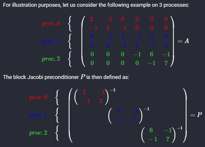
12.2 Block-Jacobi preconditioners

block Jacobi preconditioner (cnrs.fr)

the block Jacobi preconditioner:

\[P=\sum^p_{i=1}R^T_i(R_iAR^T_i)^{-1}R_i \]

where \(R_i\in \R^{n\times N}\) is the restriction matrix(取出 \(A\) 中的某一部分) from the global numbering of unknowns to the local numbering of process \(i\), and \(R_iAR^T_i\) is the diagonal block of \(A\) corresponding to the unknowns held by process \(i\).

12.3 Polynomial Preconditioners

In polynomial preconditioning hte matrix \(M\) is defined by:

\[M^{-1}=s(A) \]

12.3.2 Chebyshev Polynomials

Chebyshev Acceleration:

1. \(r_0=b-Ax_0\); \(\sigma_1=\theta/\delta\)

2. \(\rho_0=1/\sigma_1\); \(d_0=\frac1\theta r_0\)

3. For \(k=0,...,\) until convergence Do:

   1. \(x_{k+1}=x_k+d_k\)
   2. \(r_{k+1}=r_k-Ad_k\)
   3. \(\rho_{k+1}=(2\sigma_1-\rho_k)^{-1}\)
   4. \(d_{k+1}=\rho_{k+1}\rho_kd_k+\frac{2\rho_{k+1}}{\delta}r_{k+1}\)

4. EndDo

Chapter 13. Domain Decomposition Methods

new classes of numerical methods that can take better advantage of parallelism are emerging. Among these techniques, domain decomposition methods are undoubtedly the best known and perhaps the most promising for certain types of problems.

13.1 Introduction

2.2.5中有介绍不规则网格划分

13.1.1 Notation

Consider the following problem:

\[\Delta u=f\quad in\, \Omega\\ u=u_{\Gamma}\quad on\,\Gamma=\part \Omega \]

图示：

离散化之后：(the interface nodes are labeled last)

矩阵：

即：

\[\left( \begin{array}{1} B_1&&&&E_1\\ &B_2&&&E_2\\ ...&...&...&...&...\\ &&&B_s&E_s\\ F_1&F_2&...&F_s&C \end{array} \right) \left( \begin{array}{1} x_1\\x_2\\...\\x_s\\y \end{array} \right) = \left( \begin{array}{1} f_1\\f_2\\...\\f_s\\g \end{array} \right) \]

• \(x_i\) represents the subvector of unknowns that are interior to subdomain \(\Omega_i\)
• \(y\) represents the vector of all interface unknowns

即：

\[A\pmatrix{x\\y}=\pmatrix{f\\g}\quad with\,A=\pmatrix{B&E\\F&C} \]

Thus,

• \(E\) represents the subdomain to interface coupling seen from the subdomains,
• \(F\) represents the interface to subdomain coupling seen from the interface nodes.

domain decomposition or substructuring methods attempt to solve the problem on the entire domain \(\Omega=\cup \Omega_i\) from problem solutions on the subdomains \(\Omega_i\)

advantages of domain-decomposition：

• In the case of the above picture, one obvious reason is that the subproblems are much simpler because of their rectangular geometry. For example, fast solvers can be used on each subdomain in this case.
• A second reason is that the physical problem can sometimes be split naturally into a small number of subregions where the modeling equations are different (e.g., Euler’s equations on one region and Navier-Stokes in another)

13.1.2 Types of Partitionings

vertex-based partitioning：do not allow vertex to be split between two subdomains

edge-based partitioning： do not allow edges to be split between two subdomains

element-based partitioning： do not allow elements to be split between two subdomains

13.1.3 Types of Techniques

domain decomposition techniques distinguished by four features:

1. Type of Partitioning

2. Overlap

3. Processing of interface value

4. Subdomain solution. Should the subdomain problems be solved exactly or approximately by an iterative method?

本章中的methods分为：

1. direct methods and the substructuring approach are useful for introducing some definitions and for providing practical insight
2. among the simplest and oldest techniques are the Schwarz Alternating Procedures
3. based on preconditioning the Schur complement system
4. based on solving the linear system with the matrix \(A\), by using a preconditioning derived from Domain Decomposition concepts

13.2 Direct solution and the schur complement

\[x=B^{-1}(f-Ey)\quad\quad\quad\quad\quad\quad\quad (13.3)\\ (C-FB^{-1}E)y=g-FB^{-1}f\quad\quad (13.4)\\ \]

The matric \(S=C-FB^{-1}E\) is called the Schur complement matrix associated with the \(y\) variable. \((13.4)\) called the reduced system.

a solution method:

1. Obtain the right-hand side of the reduced system \((13.4)\)
2. Form the Schur complement matrix
3. Solve the reduced system \((13.4)\)
4. Back-substitute using \((13.3)\) to obtain the other unknowns.

Block-Gaussian Elimination:

1. Solve \(BE^\prime=B\), and \(Bf^\prime=f\) for \(E^\prime\) and \(f^\prime\), respectively
2. Compute \(g^\prime=g-Ff^\prime\)
3. Compute \(S=C-FE^\prime\)
4. Solve \(Sy=g^\prime\)
5. Compute \(x=f^\prime-E^\prime y\)

where:

• \(E^\prime=B^{-1}E\) and \(f^\prime =B^{-1}f\).

13.3 Schwarz alternating procedures

The original alternating procedure described by Schwarz in 1870 consisted of three parts:

• alternating between two overlapping domains
• solving the Dirichlet problem on one domain at each iteration
• taking boundary conditions based on the most recent solution obtained from other domain.

This procedure is called the Multiplicative Schwarz procedure. In matrix term, this is very reminiscent of the block Gauss-Seidel iteration with overlap defined with the help of projectors. The analogue of the block-Jacobi procedure is known as the Additive Schwarz procedure.

13.3.1 Multiplicative Schwarz Procedure

In the following, assume that each pair of neighboring subdomains has a nonvoid overlapping region. The boundary of subdomain \(\Omega_i\) that is included in subdomain \(j\) is denoted by \(\Gamma_{i,j}\).

Each subdomain extends beyond its initial boundary into nerghboring subdomains. Call \(\Gamma_i\) the boundary of \(\Omega_i\) consisting of its original boundary (which is denoted by \(\Gamma_{i,0}\)) and the \(\Gamma_{i,j}\)'s, and denote by \(u_{ji}\) the restriction of the solution \(u\) to the boundary \(\Gamma_{ji}\). Then:

Schwarz Alternating Procedure(SAP):

1. Choose an initial guess \(u\) to the solution
2. Until convergence Do:
   1. For \(i=1,...,s\) Do:
      1. Solve \(\Delta u=f\) in \(\Omega_i\) with \(u=u_{ij}\) in \(\Gamma_{ij}\)
      2. Update \(u\) values on \(\Gamma_{ji}\), \(\forall j\)
   2. EndDo
3. EndDo

The algorithm sweeps through the \(s\) subdomains and solves the original equation in each of them by using boundary conditions that are updated from the most recent values of \(u\).

we follow the model of the overlapping block-Jacobi technique seen in the previous chapter. Let \(S_i\) be an index set of subdomain:

\[S_i=\{j_1,j_2,...,j_{n_i}\},\quad \cup_{i=1,...,s}S_i=\{1,...,n\} \]

where the indices \(j_k\) are those associated with the \(n_i\) mesh points of the interior of the discrete subdomain \(\Omega_i\).

\(n_i\) 表示第 \(i\) 个subdomain包含的grid point数量.

Let:

• \(R_i\) be a restriction operator from \(\Omega\) to \(\Omega_i\). (By definition, \(x_i=R_ix\) belongs to \(Ω_i\). )（换句话说：\(R_i\) 将 \(x\) 中属于 \(\Omega_i\) 的那部分components取出来得到一个subvector）
• \(R_i^T\) the transpose is a prolongation operator which takes a variable from \(\Omega_i\) and extends it to the equivalent variable in \(\Omega\).

multiplicative Schwarz procedure:

1. For \(i=1,...,s\) Do:
   1. \(x=x+R^T_iA^{-1}_iR_i(b-Ax)\)
2. EndDo

the matrix \(A_i=R_iAR_i^T\)

个人理解：

• \(R_i(b-Ax)\): 把subdomain中的residual取出来
• \(A^{-1}_iR_i(b-Ax)\): 求出subdomain中的error
• \(R^T_iA^{-1}_iR_i(b-Ax)\): subdomain中的error扩张到全局

令error: \(d=x^\star-x\)。则在multiplicative Schwarz procedure的过程中：

\[d_i=d_{i-1}-R^T_iA^{-1}R_iAd_{i-1} \]

等价于：

\[d_i=(I-P_i)d_{i-1} \]

in which: \(P_i=R^T_iA^{-1}R_iA\)

则：

\[d_s=(I-P_s)(I-P_{s-1})...(I-P_1)d_0 \]

令：

\[Q_s=(I-P_s)(I-P_{s-1})...(I-P_1) \]

补充：restriction matrix的形式为：

13.3.2 Multiplicative Schwarz preconditioning

Proposition:

​ the multiplicative schwarz procedure is equivalent to a fixed-point iteration for the "preconditioned" problem

\[M^{-1}Ax=M^{-1}b \]

Define the matrices:

• \(T_i=P_iA^{-1}=R^T_iA^{-1}_iR_i\)

Denote:

• \(z_i=M_iv\)

Multiplicative Schwarz Preconditioner：

1. Input: \(v\); Output: \(z=M^{-1}v\)
2. \(z=T_1v\)
3. For \(i=2,...,s\) Do:
   1. \(z=z+T_i(v-Az)\)
4. EndDo

\(z_s=M^{-1}v\).

Multiplicative Schwarz Preconditioned Operator:

1. Input: \(v\), Output: \(z=M^{-1}Av\)
2. \(z=P_1v\)
3. For \(i=2,...,s\) Do
   1. \(z=z+P_i(v-z)\)
4. EndDo

14.3.3 Addtive Schwarz Procedure

​ The additive Schwarz procedure is similar to a block-Jacobi iteration and consists of updating all the new (block) components from the same residual. Thus, it differs from the multiplicative procedure only because the components in each subdomain are not updated until a whole cycle of updates through all domains are completed.

basic Addtive Schwarz iteration:

1. For \(i=1,...,s\) Do
   1. Compute \(\delta_i=R^T_iA^{-1}_iR_i(b-Ax)\)
2. EndDo
3. \(x_{new}=x+\sum^s_{i=1}\delta_i\)

Additive Schwarz Preconditioner:

1. Input: \(v\); Output: \(x=M^{-1}v\)
2. For \(i=1,...,s\) Do:
   1. Compute \(z_i=T_iv\)
3. EndDo
4. Compute \(z=z_1+z_2...+z_s\)

二，Multigrid

《A Multigrid Tutorial》2nd edition

multigrid can solve a linear system with \(N\) unknowns with only \(O(N)\) work.

多重网格法 (Multigrid Method) - 知乎

交替使用粗细网格可以解决这些迭代方法的缺陷。先在细网格上迭代使得频率大的误差衰减，剩下误差中频率较小的部分；再将误差中频率较小的部分作为方程组的右侧，在粗网格上迭代，使得频率较小的误差也能快速地衰减；最后为了保证精度，将粗网格上迭代的结果和细网格上的结果加总之后，作为初始猜测值再在细网格上迭代。如此循环往复。因为先由细到粗，后由粗到细，网格转换的路径形似 V 字，所以该方法被称为 V-Cycle Multigrid。除此之外还有 F-cycle multigrid 和 W-cycle multigrid ，基本思想都是相同。

本书的符号使用：

• We always use \(u\) to denote the exact solution of this system and \(v\) to denote an approximation to the exact solution, perhaps generated by some iterative method.
• \(\vec u\) and \(\vec v\), represent vectors, while the jth components of these vectors are denoted by \(u_j\) and \(v_j\) . In later chapters, we need to associate \(u\) and \(v\) with a particular grid： \(Ω^h\). In this case, the notation \(u^h\) and \(v^h\) is used
• error \(e=u-v\)
• residual \(r=f-Av\)，hence residual equation \(Ae=r\)
• initial guess：初始迭代值

Chapter 2. Basic Iterative Methods

详情请见上文《迭代方法》的Chapter 4.

Chapter 3. Elements of Multigrid

3.1 Move ahead multigrid

令initial guess consisting of the vectors (or Fourier modes)：由傅里叶可知，任意函数（也就是目标向量 \(v\)）可以由无数个sin函数构成

\[v_j=\sin\left(\frac{jk\pi}{n}\right) \]

\(j\)：component of vector \(v\)

\(n\)：grid node的数量

\(k\) ：wavenumber（also called frequency）

其中 \(0\le j\le n\)，\(1\le k\le n-1\)

（1）不同的frequency：

（2）不同frequency迭代的结果：

​ many standard iterative methods possess the smoothing property. This property makes these methods very effective at eliminating the high-frequency or oscillatory components of the error, while leaving the low-frequency or smooth components relatively unchanged.

​ Why use coarse grid?：Relaxation on a coarse grid is less expensive because there are fewer unknowns to be updated.

（3）对于不同密度的网格：

Through the phenomenon of aliasing, the \(k\) th mode on \(\Omega^h\) becomes the \((n-k)\)th mode on \(\Omega^{2h}\) when \(k>\frac n2\).

即：细网格高/低频，等价于粗网格低/高频 （smooth modes on a fine grid look less smooth on a coarse grid）

3.2 Transfer between fine and coarse grid

（1）fine grid to coarse grid：restriction operator \(I^{2h}_h\)

对周围点加权求和

\[I^{2h}_hv^h=v^{2h} \]

例如 \(n=8\) 时：

\[I^{2h}_hv^h=\frac14\left[ \begin{array}{1} 1&2&1&&&&\\ &&1&2&1&&\\ &&&&1&2&1 \end{array} \right] \left[ \begin{array}{1} v_1\\ v_2\\ v_3\\ v_4\\ v_5\\ v_6\\ v_7 \end{array} \right]_h =\left[ \begin{array}{1} v_1\\ v_2\\ v_3\ \end{array} \right]_{2h}=v^{2h} \]

即

\[v^{2h}=\frac14(v^h_{2j-1}+2v^h_{2j}+v^h_{2j+1}) \]

（2）coase grid to fine grid：linear interpolation operator \(I^h_{2h}\)

this is a procedure called interpolation or prolongation.

\(I^h_{2h}\) 与 \(I^{2h}_h\) 互为转置矩阵

the linear interpolation

\[I^h_{2h}v^{2h}=v^h \]

例如 \(n=8\) 时：

\[I^{h}_{2h}v^{2h}=\frac12\left[ \begin{array}{1} 1\\ 2\\ 1&1\\ &2&\\ &1&1\\ &&2\\ &&1 \end{array} \right] \left[ \begin{array}{1} v_1\\ v_2\\ v_3\ \end{array} \right]_{2h}= \left[ \begin{array}{1} v_1\\ v_2\\ v_3\\ v_4\\ v_5\\ v_6\\ v_7 \end{array} \right]_h =v^h \]

插值

3.3 Two-Grid Correction Scheme

Multigrid的两个主要步骤：

1. Relax（Smooth）：迭代解线性系统
2. correct：更新迭代的值 \(v^h\)

​ Relaxation on the original equation \(Au = f\) with an arbitrary initial guess \(v\) is equivalent to relaxing on the residual equation \(Ae = r\) with the specific initial guess \(e = 0\)

Two-grid correction（MG）的步骤：

• Relax \(ν_1\) times on \(A^hu^h = f^h\) on \(Ω^h\) with initial guess \(v^h\). （relax也可称为smoothing）//pre-smoothing
• Compute the fine-grid residual \(r^h = f^h − A^hv^h\) and restrict it to the coarse grid by \(r^{2h} = I^{2h}_h r^h\).
• Solve \(A^{2h}e^{2h} = r^{2h}\) on \(Ω^{2h}\).
• Interpolate the coarse-grid error to the fine grid by \(e^h = I^h_{2h}e^{2h}\) and correct the fine-grid approximation by \(v^h ← v^h + e^h\).
• Relax \(ν_2\) times on \(A^hu^h = f^h\) on \(Ω^h\) with initial guess \(v^h\)

上面步骤可以循环多次

• 构建grid，转换到coase grid
• 解residual equation
• 将解 \(e\) 转换到fine grid，用 \(e\) 更新 \(v\)

3.4 V-Cycle Scheme

将V-cycle（V）记作 \(v^h\leftarrow V^h(v^h,f^h)\)，则其步骤可以写为：

• Relax \(ν_1\) times on \(A^hu^h = f^h\) with initial guess \(v^h\).
• Compute \(f^{2h} = I^{2h}_h r^h=I^{2h}_h(f^h-A^hv^h)\).
  • Relax \(ν_1\) times on \(A^{2h}u^{2h} = f^{2h}\) with initial guess \(v^{2h} = 0\).
  • Compute \(f^{4h} = I^{4h}_{2h} r^{2h}\).
    • Relax \(ν_1\) times on \(A^{4h}u^{4h} = f^{4h}\) with initial guess \(v^{4h} = 0\).
    • Compute \(f^{8h} = I^{8h}_{4h} r^{4h}\).
      • · · ·
      • Solve \(A^{Lh}u^{Lh} = f^{Lh}\).
      • · · ·
    • Correct \(v^{4h} ← v^{4h} + I^{4h}_{8h} v^{8h}\).
    • Relax on \(A^{4h}u^{4h} = f^{4h}\) \(ν_2\) times with initial guess \(v^{4h}\).
  • Correct \(v^{2h} ← v^{2h} + I^{2h}_{4h} v^{4h}\).
  • Relax on \(A^{2h}u^{2h} = f^{2h}\) \(ν_2\) times with initial guess \(v^{2h}\).
• Correct \(v^h ← v^h + I^h_{2h}v^{2h}\).
• Relax on \(A^hu^h = f^h\) \(ν_2\) times with initial guess \(v^h\).

V-cycle的递归版本：

1. Relax \(ν_1\) times on \(A^hu^h = f^h\) with a given initial guess \(v^h\)
2. If \(Ω^h =\) coarsest grid, then go to step 4. Else：
   1. \(f^{2h} ← I^{2h}_h(f^h − A^hv^h)\)
   2. \(v^{2h} ← 0\)
   3. \(v^{2h} ← V^{2h}(v^{2h},f^{2h})\).
3. Correct \(v^h ← v^h + I^h_{2h}v^{2h}\).
4. Relax \(ν_2\) times on \(A^hu^h = f^h\) with initial guess \(v^h\)

3.5 \(\mu\)-cycle multigrid

\(\mu=1\) 时，等于V-cycle

将 \(\mu\)-cycle multigrid记为 \(v^{h} ← M\mu^{h}(v^{h},f^{h})\) ，则其步骤可以写为：

1. Relax \(ν_1\) times on \(A^hu^h = f^h\) with a given initial guess \(v^h\).
2. If \(Ω^h =\) coarsest grid, then go to step 4. Else：
   1. \(f^{2h} ← I^{2h}_h (f^h − A^hv^h)\)
   2. \(v^{2h} ← 0\)
   3. \(v^{2h} ← M\mu^{2h}(v^{2h},f^{2h})\) \(\mu\) times.
3. Correct \(v^h ← v^h + I^h_{2h}v^{2h}\).
4. Relax \(ν_2\) times on \(A^hu^h = f^h\) with initial guess \(v^h\)

3.6 Full Multigrid V-cycle

使用不同阶数的V-cycle组合

Full Multigrid V-cycle（FMG）记作 \(v^h\leftarrow FMG^h(f^h)\)，则其步骤：

• Initialize \(f^{2h} ← I^{2h}_h f^h, f^{4h} ← I^{4h}_{2h} f^{2h},...\)
  • Solve or relax on coarsest grid
  • · · ·
  • \(v^{2h} ← I^{2h}_{4h} v^{4h}\).
  • \(v^{2h} ← V^{2h}(v^{2h},f^{2h})\) \(ν_0\) times.
• \(v^h ← I^h_{2h}v^{2h}\).
• \(v^h ← V^h(v^h,f^h)\), \(ν_0\) times

FMG的递归版本：

1. If \(Ω^h =\) coarsest grid, set \(v^h ← 0\) and go to step 3. Else：
   1. \(f^{2h} ← I^{2h}_h (f^h)\)
   2. \(v^{2h} ← FMG^{2h}(f^{2h})\).
2. Correct \(v^h ← I^h_{2h}v^{2h}\).
3. \(v^h ← V^h(v^h,f^h)\) \(ν_0\) times.

图示：

（a）V-cycle multigrid

（b）W-cycle multigrid

（c）FMG

Chapter 4. Implementation

4.1 Data structure

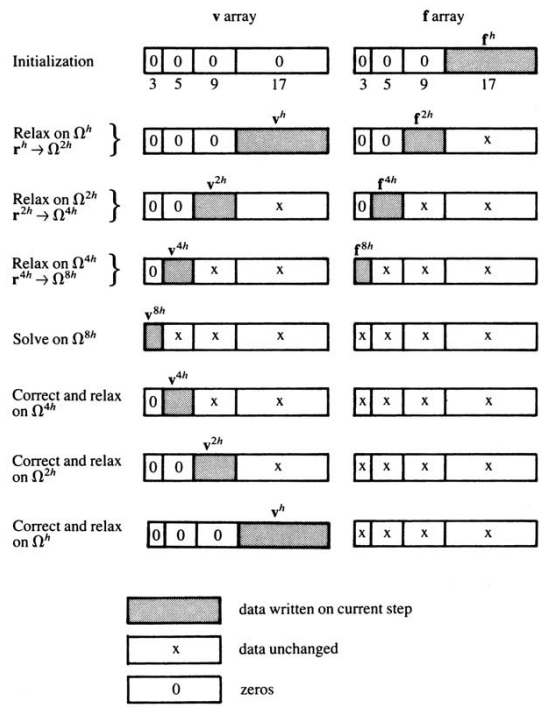
​ There seems to be general agreement that the solutions \(\vec v\) and right-side vectors \(\vec f\) on the various grids should be stored contiguously in single arrays

Consider：

• 4-level V-cycle
• 1-D problem
• \(n=16\) points

data structure的图示：

4.2 Computational cost

work unit：the cost of performing one relaxation sweep on the finest grid.

Consider：

• \(d\) dimensional V-cycle with one relaxation sweep on each level（\(v_1=v_2=1\)）.
• Each level is visited twice and grid \(\Omega^{ph}\) requires \(p^{-d}\) work units

so V-cycle computation cost：

\[=2\{1+2^{-d}+2^{-2d}+...+2^{-nd}\}<\frac2{1-2^{-d}}WU \]

example:

• 4 WUs for one-dimensional (\(d=1\)) problem
• \(8/3\) WUs for \(d=2\)
• \(16/7\) WUs for \(d=3\)

Consider：

• \(d\) dimensional FMG with one relaxation sweep on each level（\(v_0=v_1=v_2=1\)）.

so FMG computation cost：

\[=\left(\frac2{1-2^{-d}}\right)(1+2^{-d}+2^{-2d}+...+2^{-nd})<\frac2{(1-2^{-d})^2}WU \]

example:

• 8 WUs for \(d=1\)
• \(7/2\) WUs for \(d=2\)
• \(5/2\) WU for \(d=3\)

4.3 Predictive Tools: Local Mode Analysis

The remainder of this chapter presents some practical tools for determining whether an algorithm is working properly

​ 由于spectral radius难算（特征值难算），所以不容易用它分析convergence factor。所以可以使用local mode analysic (or normal mode analysis or Fourier analysis) for approximating convergence and smoothing factors.

​ Local mode analysis begins with the assumption that relaxation is a local process: each unknown is updated using information from nearby neighbors.

4.4 Diagnostic Tools

As with any numerical code, debugging can be the most difficult part of creating a successful program. For multigrid, this situation is exacerbated in two ways：

• the interactions between the various multigrid components are very subtle. It can be difficult to determine which part of a code is defective
• an incorrectly implemented multigrid code can perform quite well (sometimes better than other solution methods)

Chapter 6. Nonlinear Problems

6.1 Formal difference between linear and nonlinear

​ 书中提到nonlinear Gauss–Seidel经常用来解nonlinear system

（1）介绍：

Consider

• a system of nonlinear algebraic equations：\(A(u)=f\), where \(u,f\in R^n\) （the notation \(A(u)\), rather than \(Au\), signifies that the operator is nonlinear）

类似线性系统：

• \(e=u-v\)
• \(r=A(u)-A(v)\)

由于 \(A\) 非线性，无法推出 \(r=A(u)-A(v)=A(e)\) ，所以没有linear residual equation，now use \(r=A(u)-A(v)\) as residual equation

（2）Newton-multigrid：

residual equation等价于：

\[A(v+e)-A(v)=r \]

Expanding \(A(v+e)\) in a Taylor series about \(v\) and truncating the series after two terms, we have the linear system of equation:

\[J(v)e=r \]

where \(J=(\part A_i/\part u_j)\) is the \(n\times n\) Jacobian matrix.

​ It can be solved for \(e\) and the current approximation \(v\) can be updated by \(v\leftarrow v+e\). Iteration of this step is Newton's method. at the same time, at each step, use multigrid to solve the linear system, called Newton-multigrid.

6.2 Full Approximation Scheme（FAS）

步骤：

• Restrict the current approximation and its fine-grid residual to the coarse grid: \(r^{2h}=I^{2h}_h(f^h-A^h(v^h))\) and \(v^{2h}=I^{2h}_hv^h\)
• Solve the coarse-grid problem \(A^{2h}(u^{2h})=A^{2h}(v^{2h})+r^{2h}\)
• Compute the coarse-grid approximation to the error: \(e^{2h} = u^{2h}−v^{2h}\).
• Interpolate the error approximation up to the fine grid and correct the current fine-grid approximation: \(v^h ← v^h + I^h_{2h}e^{2h}\).

FAS can be viewed as a generalization of the two-grid correction scheme to nonlinear problems

Example：

Consider the two-point boundary value problem:

\[-u^{\prime\prime}(x)+\gamma u(x)u^\prime(x)=f(x),\quad0<x<1\\ u(0)=u(1)=0 \]

the source term \(f\) and a constant \(\gamma>0\) are given

let

• \(\Omega^h\) consist of the grid points \(x_j=\frac jn\) for some positive even integer \(n\).
• \(u_j=u(x_j)\) and \(f_j=f(x_j)\) , for \(j=0,1,...,n\).

using finite difference:

\[A^h_j(u)=\frac{-u^h_{j-1}+2u^h_j-u^h_{j+1}}{h^2}+\gamma u^h_j\left(\frac{u^h_{j+1}-u^h_{j-1}}{2h}\right)=f_j \]

​ this scalar equation is linear in \(u^h_j\) even though the vector equation \(A^h(u^h)=f^h\) is nonlinear in \(u^h\). nonlinear Gauss–Seidel requires no Newton step.

Residual equation given by:

\[A^{2h}_j(v^{2h}+e^{2h})-A^{2h}_j(v^{2h})=r^{2h}_j \]

把Residual equation中的 \(A^{2h}_j\) 用上面finite difference的 \(A^h_j(u)\) 做替换

Chapter 7. Multigrid preconditioning

multigrid可以被用作preconditioner

​ If the matrix of the original equation or an eigenvalue problem is symmetric positive definite (SPD), the preconditioner is commonly constructed to be SPD as well, so that conjugate gradient can still be used.

​ When using multigrid as a preconditioner, the action of this preconditioner is obtained by applying a fixed number of multigrid cycles.

Multigrid做standalone solver就是解到哪里算哪里，留下的residual通通不管；做Preconditioner的话，你的residual会根据你是用的krylov solver的特性继续减小。

7.1 MGPCG

MST10.pdf (ucla.edu) : A parallel multigrid Poisson solver for fluids simulation on large grids

MGPCG:

V-Cycle Algorithm:

Smoother:

Chapter 8. Algebraic Multigrid（AMG）

论文《An Introduction to Algebraic Multigrid》

8.1 Introduction

介绍：

• algebraic multigrid methods (AMG) construct their hierarchy of operators directly from the system matrix. （The AMG method determines coarse “grids”, inter-grid transfer operators, and coarse-grid equations based solely on the matrix entries）

• In classical AMG, the levels of the hierarchy are simply subsets of unknowns without any geometric interpretation.Thus, AMG methods become black-box solvers for certain classes of sparse matrices

• requires no explicit knowledge of the problem geometry（ Since AMG knows nothing about the geometry of the problem, we need to characterize this in some algebraic way）

前文中的插值矩阵 \(I_{2h}^h\) 重新记为 \(P\)，则 \(I^{2h}_h\) 记为 \(P^T\)

Because AMG is based only on the matrix \(A\), there are few options for defining the coarse system \(A_c\). The most common approach is to use the Galerkin operator：

\[A_c=P^TAP \]

8.1.1 Adjacency graph

fine-grid：soving \(Au=f\), where \(u=[u_1...u_n]\). Then the fine-grid points are just the indices \({1, 2,...,n}\).

​ the connections within the grid are determined by the undirected adjacency graph of the matrix：

The connections in the grid are the edges in the graph

The grid in AMG is simply the set of vertices in the graph（grid point \(i\) is just vertex \(i\)）

8.1.2 Algebraic smoothness

​ If the problem provides no geometric information, then we cannot simply examine the Fourier modes of the error.

​ we define smooth error loosely to be any error that is not reduced effectively by relaxation. （例如：粗网格上迭代高频，细网格上迭代低频，会导致error无法下降）

​ Weighted Jacobi relaxation, as we know, has the property that after making great progress toward convergence, it stalls, and little improvement is made with successive iterations. At this point, we define the error to be algebraically smooth. （By our definition, algebraic smoothness means that the size of \(e^{i+1}\) is not significantly less than that of \(e^i\)，也就是：第 \(i+1\) 次迭代后error不一定别第 \(i\) 次小）

8.1.3 Influence and Dependence

（1）Dependence：

Given a threshold value \(0 < θ ≤ 1\), the variable (point) \(u_i\) strongly depends on the variable (point) \(u_j\) if

\[−a_{ij} ≥ θ \max_{k\ne i} \{−a_{ik}\} \]

This says that grid point \(i\) strongly depends on grid point \(j\) if the coefficient \(a_{ij}\) is comparable in magnitude to the largest off-diagonal coefficient in the \(i\)th equation

（2）Influence：

If the variable \(u_i\) strongly depends on the variable \(u_j\) , then the variable \(u_j\) strongly influences the variable \(u_i\).

8.1.4 Defining the Interpolation Operator

​ The coarsening procedure partitions the grid into C-points (points on the coarse grid) and F-points (points not on the coarse grid (only on the fine-grid) )

​ For each fine-grid point \(i\), we define \(N_i\), the neighborhood of \(i\), to be the set of all points \(j\ne i\) such that \(a_{ij} \ne 0\). These points can be divided into three categories:

• the neighboring coarse-grid points that strongly influence \(i\); this is the coarse interpolatory set for \(i\), denoted by \(C_i\).

• the neighboring fine-grid points that strongly influence \(i\), denoted by \(D^s_i\).

• the points that do not strongly influence \(i\), denoted by \(D^w_i\) ; this set may contain both coarse- and fine-grid points; it is called the set of weakly connected neighbors.

smooth error that must be interpolated to the fine grid：

\[(I^h_{2h}e)_i=\left\{ \begin{array}{1} e_i &if\quad i\in C\\ \sum_{j\in{C_i}}\omega_{ij}e_j&if\quad i\in F \end{array} \right. \]

8.1.5 Selecting the Coarse Grid

8.2 Classical AMG

（1）Choosing the coarse grid：

1. Define a strength matrix \(A_s\) by deleting weak connections in \(A\).
2. First pass：Choose an independent set of fine-grid points based on the graph of \(A_s\).
3. Second pass：Choose additional points if needed to satisfy interpolation requirements.

8.3 AMG Two-Grid correction cycle

步骤：

• Relax \(\nu_1\) times on \(A^hu^h=f^h\) with initial guess \(v^h\).
• Compute the fine-grid residual \(r^h = f^h − A^hv^h\) and restrict it to the coarse grid by \(r^{2h} = I^{2h}_h r^h\).
• Solve \(A^{2h}e^{2h} = r^{2h}\) on \(Ω^{2h}\).
• Interpolate the coarse-grid error to the fine grid by \(e^h = I^h_{2h}e^{2h}\) and correct the fine-grid approximation by \(v^h ← v^h + e^h\).
• Relax \(ν_2\) times on \(A^hu^h = f^h\) with initial guess \(v^h\).

Chapter 9. Multilevel Adaptive Methods

The goal of this chapter is to understand how to treat local demands in a multilevel context without overburdening the overall computation. （不需要全部计算，即可针对性地解决某个local demands）

9.1 Introduction

​ To keep matters simple, assume that a local fine grid with mesh size \(h = \frac18\) is needed on the interval \((\frac12,1)\) to resolve some special feature near \(x = \frac34\) , but that a mesh size of \(2h = \frac14\) is deemed adequate for the rest of the domain. （要solve some special feature near \(x=\frac34\)，需要 \((\frac12,1)\) 区间的网格的密度达到 \(h=\frac18\)，剩下的 \((0,\frac12)\) 区间的网格密度只需要达到 \(2h=\frac14\) 即可）

思路：

• 对于非local fine grid，不做relax，直接将residual给restrict到coarse grid.
  • residual给restrict到coarse grid之后，下一轮直接更新coarse grid的residual即可
• 对于local fine grid，正常走流程
• 在coarse grid中，通过对residual equation的relax求得error，然后将error插值回到fine grid，再进行correct

由于非local fine grid在fine grid上不做relax，所以可以用参数 \(\omega\) 来累积coarse grid solution

9.2 Fast Adaptive Composite Grid Method（FAC）

• Initialize \(v^h = 0, w^{2h}_1 = 0\), and \(f^{2h}_1 ≡ (I^{2h}_h f^h)_1 = \frac{f^h_1 +2f^h_2 +f^h_3}4\) .
• Relax on \(v_h\) on the local fine grid \(\{x^h_5 , x^h_6 , x^h_7\} = \{ \frac58 , \frac34 , \frac78 \}\).
• Compute the right sides for the local coarse grid: \(f^{2h}_2 ← g^{2h}_2 − \frac{−w^{2h}_1 +2v^h_4 −v^h_6} {(2h)^2}\) , \(f^{2h}_3 ← \frac{r^h_5 +2r^h_6 +r^h_7}4\) .
• Compute an approximation \(v^{2h}\) to the coarse-grid residual equation \(A^{2h}u^{2h} = f^{2h}\).
• Update the residual at \(× = \frac14\) for use in later cycles: \(f^{2h}_1 ← f^{2h}_1 −\frac{−v^{2h}_0 +2v^{2h}_1 −v^{2h}_2} {(2h)^2}\) .
• Update the coarse-grid approximation at \(× = \frac14: w^{2h}_1 ← w^{2h}_1 + v^{2h}_1\) .
• Interpolate the correction and update the approximation: \(v^h ← v^h + I^h_{2h}v^{2h}\) at the local fine grid and the interface points \(\{ \frac12 , \frac58 , \frac34 , \frac78 \}\).

补充概念：

流体

Warm starting：use the \(p\) from the last frame as the initial guess of the current frame. （\(p\) 为流体的压强场）（对MGPCG效果不太好，对其它方法效果好）

为什么使用multigrid：discretization的时候，中间的cell对周围4个cell做discretization (比如说finite difference)，这个linear operator可以看到的cell只有5个，是比较high frequency的，而速度的divergence可能是一个large scale, low frequency的，就没有办法被capture到。（在CG中，很少用来做solver，而是做preconditioner）（通常，multigrid每次迭代residual都是降低一个数量级）

Papers:

• (sig2018) An Advection-Reflection Solver for Detail-Preserving Fluid Simulation